スケールをまたぐエルゴード性の発現
このノートブックでは、Onset of Ergodicity Across Scales on a Digital Quantum Processor [arXiv:2603.12236] の実験を実行・解析する方法を順に説明します。モデルから回路へ、ビット列からエントロピーへ、ノイズを含むデータから緩和された結果へ、そして16量子ビットのシミュレーションからIBM Quantum® Nighthawkプロセッサ上の64量子ビットの実行へと進みます。コードはすべてここにあり、各関数は最初に必要になる箇所で定義されます。
| 時間 | セクション |
|---|---|
| 0–1分 | セットアップ |
| 1–6分 | 1. モデルから回路へ |
| 6–12分 | 2. 何を測定し、どのように推定するか |
| 12–19分 | 3. ノイズと、その取り除き方 |
| 19–24分 | 4. 大規模な実行 |
| 24–33分 | 5. ハードウェアのデータ |
| 33–35分 | まとめ |
進め方。 セルを上から順に実行してください。IBM Quantumのアカウントは不要です。ハードウェアジョブを送信するセルはオフになっており、セクション5では保存済みのハードウェア実行を解析します。これはセットアップセルが data/ にダウンロードします。ディスカッション用の質問には Question と記されています。答えを開く前に答えてみてください。
セットアップ
Python 3.12以降と、次のパッケージが必要です。
-
Qiskit SDK v2.5以降(可視化サポート付き)
-
Qiskit Runtime v0.49以降(
pip install qiskit-ibm-runtime) -
Qiskit Aer v0.17以降(
pip install qiskit-aer) -
Samplomatic v0.21以降(
pip install samplomatic) -
NumPyとMatplotlib
セットアップセルは、保存済みのハードウェア実行とMPS参照データ(約9 MB)も、まだ data/ にない場合はそこにダウンロードします。
# Added by doQumentation — installs the packages this notebook needs if they are missing
import importlib.util

_needed = {"matplotlib": "matplotlib", "numpy": "numpy", "qiskit": "qiskit", "qiskit_aer": "qiskit-aer", "qiskit_ibm_runtime": "qiskit-ibm-runtime", "samplomatic": "samplomatic"}
_missing = [pip for module, pip in _needed.items()
            if importlib.util.find_spec(module) is None]
# One at a time, so a package that fails to install does not block the others
for _pip in _missing:
    %pip install -q {_pip}
if not _missing:
    print("\u2713 All required packages are installed")
from math import comb
from pathlib import Path
from urllib.request import urlretrieve

import matplotlib.pyplot as plt
import numpy as np
from qiskit import ClassicalRegister, QuantumCircuit, QuantumRegister
from qiskit.primitives import StatevectorSampler
from qiskit.quantum_info import (
    PauliLindbladMap,
    QubitSparsePauli,
    Statevector,
)
from qiskit.transpiler import generate_preset_pass_manager
from qiskit_aer import AerSimulator
from qiskit_aer.noise import NoiseModel, ReadoutError, depolarizing_error
from qiskit_aer.primitives import SamplerV2 as AerSampler

RUN_ON_HARDWARE = (
    False  # True submits the 8x8 jobs in section 4 (needs Nighthawk access)
)
COMPUTE_MPS_REFERENCES = False  # True recomputes the MPS references in section 5 (about 18 minutes)

# Download the saved hardware run and MPS references, unless they are already in data/
data_url = "https://raw.githubusercontent.com/Qiskit/documentation/main/datasets/tutorials/onset-of-ergodicity"
Path("data").mkdir(exist_ok=True)
for name in ("hardware_run.npz", "mps_references_all.npz"):
    if not Path("data", name).exists():
        urlretrieve(f"{data_url}/{name}", Path("data", name))
1. モデルから回路へ
2量子ビット・ゲート
格子のすべての結合 に同じ2量子ビット・ゲートが適用されます。このゲートは、ハイゼンベルク・エンタングラーとそれに続くランダム場からなります。
ここで は、ゲートごとに から一様に選ばれます。
Question. を、ハードウェアが実行できるゲートにどのように分解しますか?
答え
場は簡単です。 は、各量子ビットに対する1量子ビット回転 です。
エンタングラーが難しい部分です。、、 は可換なので、3つの回転 、、 に因数分解できます。それぞれにCNOTが2つ必要なので、ゲートあたりCNOTは6つになります。
もっと良い方法があります。任意の2量子ビット・ゲートは、最大3つのCNOTと1量子ビット回転で構成できます。最適な回路は の形から始まり、このエンタングラーは としてすでにその形をしています。したがって、そのまま3つのCNOTに対応づけられ、1量子ビットの角度は について線形です。実験コードはこの方法でゲートを構築しています。
ハードウェアでは、2量子ビット・ゲートごとにノイズが加わるため、CNOTの数を半分にすることが重要です。
def xxyyzz_gate(circuit, coupling, i, j):
    # exp(iJ(XX + YY + ZZ)) with three CNOTs; only the rotation angles depend on J
    circuit.rz(-np.pi / 2, j)
    circuit.cx(j, i)
    circuit.rz(np.pi / 2 - 2 * coupling, i)
    circuit.ry(2 * coupling - np.pi / 2, j)
    circuit.cx(i, j)
    circuit.ry(np.pi / 2 - 2 * coupling, j)
    circuit.cx(j, i)
    circuit.rz(np.pi / 2, i)

def heisenberg_gate(circuit, coupling, i, j, h_i, h_j):
    # The entangler first, then the random fields exp(i h Z)
    xxyyzz_gate(circuit, coupling, i, j)
    circuit.rz(-2 * h_i, i)
    circuit.rz(-2 * h_j, j)

h_i, h_j = 0.3, -0.7
gate = QuantumCircuit(2)
heisenberg_gate(gate, 0.05 * np.pi, 0, 1, h_i, h_j)
gate.draw("mpl")

ブリックワークとFloquetサイクル
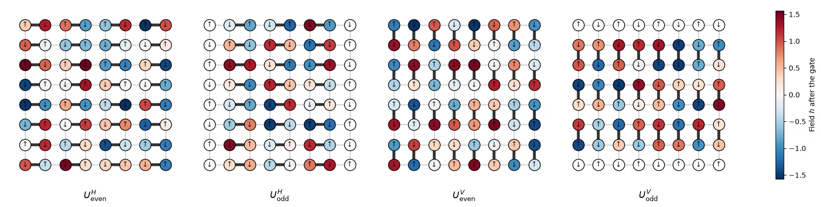
ゲートは、重ならない結合からなる4つのサブレイヤーで正方格子を敷き詰めます(ブリックワーク)。偶数列から始まる水平結合、次に奇数列、続いて偶数行から始まる垂直結合、次に奇数行の順です。量子ビット はサイト に位置します。
def brickwork_layers(num_cols, num_rows):
    # Bonds of the square lattice, in the four sublayers of the brickwork
    def qubit(x, y):
        return y * num_cols + x

    layers = []
    for p in (0, 1):  # horizontal bonds starting on even, then odd, columns
        layers.append(
            [
                (qubit(x, y), qubit(x + 1, y))
                for y in range(num_rows)
                for x in range(p, num_cols - 1, 2)
            ]
        )
    for p in (0, 1):  # vertical bonds starting on even, then odd, rows
        layers.append(
            [
                (qubit(x, y), qubit(x, y + 1))
                for y in range(p, num_rows - 1, 2)
                for x in range(num_cols)
            ]
        )
    return layers

brickwork_layers(4, 4)
[[(0, 1), (2, 3), (4, 5), (6, 7), (8, 9), (10, 11), (12, 13), (14, 15)],
 [(1, 2), (5, 6), (9, 10), (13, 14)],
 [(0, 4), (1, 5), (2, 6), (3, 7), (8, 12), (9, 13), (10, 14), (11, 15)],
 [(4, 8), (5, 9), (6, 10), (7, 11)]]
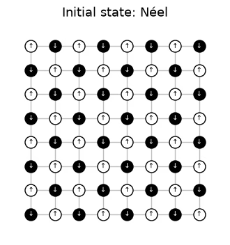
4つのサブレイヤーで1つのFloquetサイクルになります。このサイクルは同じ場で 回繰り返されるため、ダイナミクスは空間的にはランダムで、時間的には周期的です。回路はネール状態から始まり、 は格子の一辺の長さの半分です。 次のセルは、論文の図5のスタイルで、ハードウェア実行の場を使って、 のハードウェア格子の1つのFloquetサイクルをサブレイヤーごとに描画します。太い結合は各サブレイヤーのゲートです。ゲートが作用する各量子ビットは、その後に受け取るランダム場 で色分けされ、アイドル状態の量子ビットは白です。矢印はネール初期状態を示し、 は を表します。論文の図では垂直サブレイヤーが先に適用されますが、どちらの順序でも物理は変わらないと考えられます。
# circuit structure, 8x8 system:
side = 8
all_bonds = [bond for layer in brickwork_layers(side, side) for bond in layer]

# get the disorder parameters for a given system:
def sample_disorder(num_cols, num_rows, rng):
    # One pair of fields (h_i, h_j) per gate, reused in every Floquet cycle
    return [
        [
            (bond, tuple(rng.uniform(-np.pi / 2, np.pi / 2, 2)))
            for bond in layer
        ]
        for layer in brickwork_layers(num_cols, num_rows)
    ]

# build the structure for the 8x8 system
example_disorder = sample_disorder(
    side, side, np.random.default_rng(7)
)  # the hardware fields (section 4)
titles = [
    r"$U^H_\mathrm{even}$",
    r"$U^H_\mathrm{odd}$",
    r"$U^V_\mathrm{even}$",
    r"$U^V_\mathrm{odd}$",
]
norm = plt.Normalize(-np.pi / 2, np.pi / 2)
cmap = plt.get_cmap("RdBu_r")

fig, axes = plt.subplots(1, 4, figsize=(16, 4.8), layout="constrained")
for ax, title, sublayer in zip(axes, titles, example_disorder):
    for i, j in all_bonds:
        ax.plot(
            [i % side, j % side],
            [i // side, j // side],
            color="0.75",
            lw=1,
            zorder=0,
        )
    fields = {}
    for (i, j), (h_i, h_j) in sublayer:
        ax.plot(
            [i % side, j % side],
            [i // side, j // side],
            color="0.2",
            lw=4,
            zorder=1,
        )
        fields[i], fields[j] = h_i, h_j
    for q in range(side * side):
        x, y = q % side, q // side
        ax.scatter(
            x,
            y,
            s=260,
            color=cmap(norm(fields[q])) if q in fields else "white",
            edgecolor="black",
            zorder=2,
        )
        ax.text(
            x,
            y,
            "↓" if (x + y) % 2 else "↑",
            ha="center",
            va="center",
            fontsize=9,
            zorder=3,
        )
    ax.set_aspect("equal")
    ax.set_xlim(-1, side)  # padding, so the panels read as separate steps
    ax.set_ylim(side, -1)
    ax.axis("off")
    ax.set_title(title, y=-0.1, fontsize=13)
fig.colorbar(
    plt.cm.ScalarMappable(norm=norm, cmap=cmap),
    ax=axes,
    shrink=0.7,
    label="Field $h$ after the gate",
)
plt.show()
初期状態を定義します。
# initial state
def neel_state(circuit, num_cols, num_rows, layout):
    for y in range(num_rows):
        for x in range(num_cols):
            if (x + y) % 2 == 1:
                circuit.x(layout[y * num_cols + x])
# The initial Néel state: |1⟩ (black, ↓) on odd sites, |0⟩ (white, ↑) on even sites

fig, ax = plt.subplots(figsize=(4, 4.4))
for i, j in all_bonds:
    ax.plot(
        [i % side, j % side],
        [i // side, j // side],
        color="0.75",
        lw=1,
        zorder=0,
    )
for q in range(side * side):
    x, y = q % side, q // side
    excited = (x + y) % 2 == 1
    ax.scatter(
        x,
        y,
        s=150,
        color="black" if excited else "white",
        edgecolor="black",
        zorder=2,
    )
    ax.text(
        x,
        y,
        "↓" if excited else "↑",
        ha="center",
        va="center",
        fontsize=7,
        color="white" if excited else "black",
        zorder=3,
    )
ax.set_aspect("equal")
ax.set_xlim(-1, side)
ax.set_ylim(side, -1)
ax.axis("off")
ax.set_title("Initial state: Néel", fontsize=13)
plt.show()
# actual circuit construction:
def heisenberg_floquet_circuit(
    num_cols, num_rows, coupling, num_cycles, disorder, measure=True
):
    num_qubits = num_cols * num_rows
    circuit = QuantumCircuit(num_qubits)
    neel_state(circuit, num_cols, num_rows, list(range(num_qubits)))
    cycle = QuantumCircuit(num_qubits)
    for sublayer in disorder:
        for (i, j), (h_i, h_j) in sublayer:
            heisenberg_gate(cycle, coupling, i, j, h_i, h_j)
    for _ in range(num_cycles):
        circuit.compose(cycle, inplace=True)
    if measure:
        circuit.measure_all()
    return circuit
の例
シミュレーションでは、2サイクルの 格子と、論文で研究されている結合 を使用します。1組の場がすべての結合で再利用されます。
# simulation parameters:
num_cols = num_rows = 4
num_qubits = num_cols * num_rows
num_cycles = 2
couplings = (
    np.array([0.005, 0.01, 0.02, 0.03, 0.04, 0.05, 0.06, 0.08, 0.10, 0.125])
    * np.pi
)
disorder = sample_disorder(num_cols, num_rows, np.random.default_rng(42))

# circuit construction:
logical_circuits = [
    heisenberg_floquet_circuit(
        num_cols, num_rows, coupling, num_cycles, disorder
    )
    for coupling in couplings
]
logical_circuits[5].draw(output="mpl", fold=-1)

# transpiling the circuit:
pass_manager = generate_preset_pass_manager(
    optimization_level=3,
    basis_gates=["cz", "rz", "sx", "x"],
    seed_transpiler=7,
)
circuits = [pass_manager.run(circuit) for circuit in logical_circuits]

def two_qubit_stats(circuit):
    count = sum(1 for inst in circuit.data if inst.operation.num_qubits == 2)
    depth = circuit.depth(lambda inst: inst.operation.num_qubits == 2)
    return count, depth

stats = {two_qubit_stats(circuit) for circuit in circuits}
assert len(stats) == 1, "the CZ structure should not depend on J"
num_cz, depth = stats.pop()
print(
    f"{num_qubits} qubits: {num_cz} CZ gates in {depth} layers, for every coupling"
)
circuits[5].draw("mpl", fold=-1, scale=0.4)
16 qubits: 144 CZ gates in 24 layers, for every coupling

回路(と実験)はIBM Nighthawk向けに設計されているため、高度なコンパイラは必要ありません。
格子をシミュレーションする
格子では、両方を行えます。すべての結合で厳密な状態を計算することと、実験と同じように、すべての回路を10,000ショットでサンプリングすることです。ショットは(バッチ、ショット、量子ビット)という形状で保存され、これはハードウェアデータのランダム化と同じレイアウトです。ここでは10,000ショットすべてが1つのバッチを構成するため、バッチに対するブートストラップはショットノイズを加えず、次のプロットの誤差バーは周辺分布の位置間のばらつきのみを示します。
exact_states = [
    Statevector(
        heisenberg_floquet_circuit(
            num_cols, num_rows, c, num_cycles, disorder, measure=False
        )
    )
    for c in couplings
]

shots = 10_000
results = (
    StatevectorSampler(default_shots=shots, seed=1234).run(circuits).result()
)

# the output of the simulation for the 10 couplings
bits = [
    result.data.meas.to_bool_array(order="little").reshape(
        1, 10_000, num_qubits
    )
    for result in results
]

print(bits[0])
[[[False  True False ... False  True False]
  [False  True False ... False  True False]
  [False  True False ... False  True False]
  ...
  [False  True False ... False  True False]
  [False  True False ... False  True False]
  [False  True False ... False  True False]]]
2. 何を測定し、どのように推定するか
IPRと衝突エントロピー
個の量子ビットからなる周辺分布 について、ビット列の分布を とすると、推定すべき量は周辺分布の逆参加比(IPR)であり、そこから衝突エントロピーが得られます。
は、2つのショットが周辺分布上で一致する確率でもあります。積状態では 、ランダム状態では なので、周辺分布がランダムになるにつれて、 は0から約 ビットまで上昇します。
推定量1: ショットのペアを数える
Question. ショットからこの量をどのように推定しますか?
答え
素朴な推定量では、ショットから各 を として計算し、 を求めます。 この推定量にはバイアスがあります。
はすべてのショットを自分自身と一致するものとして数えるため、推定値が押し上げられます。平均すると、 ではなく が得られます。 は2つのショットが一致する確率なので、異なるショットのペアだけを数えます。
これは不偏であり、以下の ipr_from_shots が計算しているものです。
# IPR expectation values:

# refactor this function cause it does not scale
def ipr_from_shots(bits):
    # Pair-counting estimate of the IPR of a marginal: the fraction of pairs of different shots
    # that agree on it. bits holds the marginal's qubits only, with shape (randomizations, shots,
    # qubits), and all randomizations are pooled.
    n = bits.shape[-1]
    outcomes = bits @ 2 ** np.arange(
        n
    )  # each shot's marginal bitstring, read as an integer
    counts = np.bincount(outcomes.ravel())  # how often each outcome occurs
    total = counts.sum()
    return float((counts * (counts - 1)).sum() / (total * (total - 1)))

def collision_entropy(ipr):
    return -np.log2(ipr)
推定量2: パーセバル展開
IPRは、周辺分布の空でないすべての部分集合 のパリティ を使って表すこともできます。
PEAなどのエラー緩和手法は確率ではなく期待値に対して働くため、この形は重要です。 1量子ビット: 測定結果の確率は と なので、
の周辺分布: 量子ビットに とラベルを付けると、周辺分布には 個のパリティがあります。単一量子ビットが4つ、ペアが6つ、3つ組が4つ、そして周辺分布全体です。したがって、
def parity_supports(patch):
    # All nonempty subsets S of the marginal
    return sorted(
        [
            tuple(q for k, q in enumerate(patch) if mask & (1 << k))
            for mask in range(1, 1 << len(patch))
        ],
        key=len,
    )

def parity_expectation_values(bits, supports):
    # Shot-averaged <Z_S> for every support, per randomization
    signs = 1 - 2 * bits.astype(np.int8)
    return np.stack(
        [signs[..., list(s)].prod(axis=-1).mean(axis=-1) for s in supports],
        axis=-1,
    )

# Example: the parities of a 3-qubit marginal made of lattice qubits 5, 6, and 9
print(parity_supports([5, 6, 9]))
print(f"A 3×3 marginal has {len(parity_supports(range(9)))} parities")
[(5,), (6,), (9,), (5, 6), (5, 9), (6, 9), (5, 6, 9)]
A 3×3 marginal has 511 parities
周辺分布にわたる平均
追加の便利な関数: ハール値、周辺分布の選択、ブートストラップ、平均化。
# functions for the Haar values on plots:
def haar_ipr(num_patch, num_qubits):
    # Mean IPR of a marginal for Haar-random states in the sector with num_qubits // 2 ones
    weight = num_qubits // 2
    dimension = comb(num_qubits, weight)
    total = 0
    for k in range(num_patch + 1):  # k ones on the marginal
        rest = (
            comb(num_qubits - num_patch, weight - k) if weight - k >= 0 else 0
        )
        total += comb(num_patch, k) * rest * (rest + 1)
    return total / (dimension * (dimension + 1))

def haar_entropy(num_patch, num_qubits):
    return collision_entropy(haar_ipr(num_patch, num_qubits))

# definitions of positions in the lattice:
def patch_qubits(anchor, shape, num_cols):
    # Lattice indices of a rectangular marginal with its top-left corner at anchor
    (x0, y0), (width, height) = anchor, shape
    return [
        (y0 + dy) * num_cols + (x0 + dx)
        for dy in range(height)
        for dx in range(width)
    ]

def all_positions(shape, num_cols, num_rows):
    # Every placement of a (width, height) marginal on the lattice
    width, height = shape
    return [
        patch_qubits((x, y), shape, num_cols)
        for y in range(num_rows - height + 1)
        for x in range(num_cols - width + 1)
    ]

# bootstrapping for error bars:
bootstrap_rng = np.random.default_rng(0)

def bootstrap_error(statistic, *samples, axis=0, num_resamples=50):
    # Shot noise of a statistic, from resampling the randomizations (along axis of every
    # sample) with replacement
    values = []
    for _ in range(num_resamples):
        resampled = [
            np.take(
                x,
                bootstrap_rng.integers(0, x.shape[axis], x.shape[axis]),
                axis=axis,
            )
            for x in samples
        ]
        values.append(statistic(*resampled))
    return float(np.std(values, ddof=1))

# averaging the ipr over marginals:
def average_ipr(iprs, shot_errors):
    # iprs and shot_errors have shape (positions, couplings). The mean IPR over positions, and its
    # error: the spread between positions plus the shot noise of each (law of total variance)
    iprs, shot_errors = np.asarray(iprs), np.asarray(shot_errors)
    count = len(iprs)
    variance = (
        iprs.var(axis=0, ddof=1) / count
        + (shot_errors**2).sum(axis=0) / count**2
    )
    return iprs.mean(axis=0), np.sqrt(variance)
# Calculating exact simulation entropies:
patch_shapes = {
    "1×1": (1, 1),
    "1×2": (2, 1),
    "2×2": (2, 2),
    "2×3": (3, 2),
    "3×3": (3, 3),
}

# calculate the exact entropies:
sim_positions = {
    label: all_positions(shape, num_cols, num_rows)
    for label, shape in patch_shapes.items()
}
exact_iprs = {  # shape (positions, couplings)
    label: np.array(
        [
            [(s.probabilities(qargs=q) ** 2).sum() for s in exact_states]
            for q in qubit_lists
        ]
    )
    for label, qubit_lists in sim_positions.items()
}
exact_entropies = {
    label: collision_entropy(v.mean(axis=0))
    for label, v in exact_iprs.items()
}

# Average IPR of every shape over its positions, from the sampled shots, then the entropy
iprs_from_shots = {}  # per shape: average IPR and its error, at every coupling
entropies_from_shots = {}  # per shape: average entropy and its error, at every coupling
for label, qubit_lists in sim_positions.items():
    iprs = [[ipr_from_shots(b[:, :, q]) for b in bits] for q in qubit_lists]

    # bootstrapping over subsampling for error bars:
    errors = [
        [bootstrap_error(ipr_from_shots, b[:, :, q]) for b in bits]
        for q in qubit_lists
    ]
    ipr, ipr_error = average_ipr(iprs, errors)
    iprs_from_shots[label] = (ipr, ipr_error)
    entropies_from_shots[label] = (
        collision_entropy(ipr),
        ipr_error / (ipr * np.log(2)),
    )
# Now plot the average IPR on the left, and the same averages as entropies on the right
colors = plt.cm.plasma(np.linspace(0.05, 0.8, len(patch_shapes)))
fig, (ax_ipr, ax_entropy) = plt.subplots(1, 2, figsize=(12.8, 4.2))
for (label, qubit_lists), color in zip(sim_positions.items(), colors):
    n = len(qubit_lists[0])
    ipr, ipr_error = iprs_from_shots[label]
    entropy, entropy_error = entropies_from_shots[label]
    # Left: the average IPR, with its exact value and its random-state value
    ax_ipr.axhline(haar_ipr(n, num_qubits), color=color, ls="dashdot", lw=0.9)
    ax_ipr.plot(
        couplings / np.pi, exact_iprs[label].mean(axis=0), color=color
    )
    ax_ipr.errorbar(
        couplings / np.pi,
        ipr,
        yerr=ipr_error,
        fmt="o",
        color=color,
        mec="white",
        ms=7,
        capsize=3,
        label=f"{label} ({len(qubit_lists)} positions)",
    )
    # Right: the average collision entropy
    ax_entropy.axhline(
        haar_entropy(n, num_qubits), color=color, ls="dashdot", lw=0.9
    )
    ax_entropy.plot(couplings / np.pi, exact_entropies[label], color=color)
    ax_entropy.errorbar(
        couplings / np.pi,
        entropy,
        yerr=entropy_error,
        fmt="o",
        color=color,
        mec="white",
        ms=7,
        capsize=3,
        label=f"{label} ({len(qubit_lists)} positions)",
    )
ax_ipr.set_yscale("log")
ax_ipr.set_ylabel("Average IPR")
ax_entropy.set_ylabel("Average collision entropy (bits)")
for ax in (ax_ipr, ax_entropy):
    ax.set_xlabel("Coupling $J/\\pi$")
fig.suptitle("Exact (lines) and sampled (dots), 4×4 lattice, 2 cycles")
ax_entropy.legend(title="Marginal", loc="upper left")
fig.tight_layout()
plt.show()
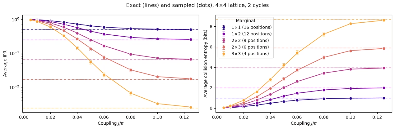
どの周辺分布の形状も、ランダム状態の値に向かって滑らかに上昇し、より大きな周辺分布ほどより大きな でそこに到達します。
3. ノイズと、その取り除き方
ノイズのあるシミュレーション
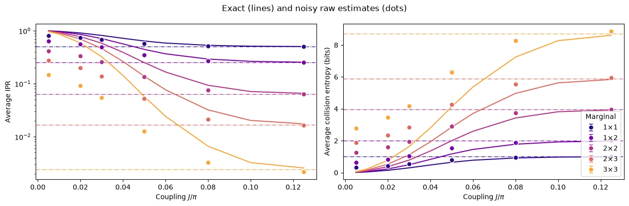
ここでノイズを加えます。すべてのCZゲートに1%の2量子ビット脱分極ノイズ、すべての量子ビットに3%の読み出しエラーを加え、Qiskit Aer Samplerでサンプリングします。回路には144個のCZゲートがあり、8×8のハードウェア回路が受けるノイズよりはるかに小さいものの、その影響を見るには十分です。このシミュレーションでは6つの結合をそれぞれ4,000ショットで使用し、約1.5分かかります。
Question. 実行する前に考えてみてください。ノイズは、系をより熱平衡化したように見せるでしょうか、それとも熱平衡化していないように見せるでしょうか?
答え
より熱平衡化したように見えます。ノイズは測定結果を乱し、すべての周辺分布を一様分布に近づけるため、生のIPRは下がり、エントロピーは上がります。緩和しなければ、ノイズは存在しない熱平衡化のように見え、クロスオーバーが早すぎる位置に現れます。
# define the noise model

noise_model = NoiseModel()
# two qubit depolarizing noise:
noise_model.add_all_qubit_quantum_error(depolarizing_error(0.01, 2), ["cz"])
# symmetric readout noise:
noise_model.add_all_qubit_readout_error(
    ReadoutError([[0.97, 0.03], [0.03, 0.97]])
)

# simulation is done using trajectories
noisy_sampler = AerSampler(
    default_shots=4000,
    seed=1,
    options={"backend_options": {"noise_model": noise_model}},
)

# choose a subset of J values for speed:
noisy_indices = [
    0,
    2,
    3,
    5,
    7,
    9,
]  # J/π = 0.005, 0.02, 0.03, 0.05, 0.08, 0.125
noisy_results = noisy_sampler.run(
    [circuits[k] for k in noisy_indices]
).result()

# No twirling here, so the 20 "randomizations" are just batches of 200 shots
noisy_bits = {
    k: result.data.meas.to_bool_array(order="little").reshape(
        20, 200, num_qubits
    )
    for k, result in zip(noisy_indices, noisy_results)
}
# Calculating noisy entropies

# Average IPR of every shape over its positions, from the noisy shots, then the entropy
noisy_iprs = {}  # per shape: average IPR and its error, at every noisy coupling
noisy_entropies = {}  # per shape: average entropy and its error, at every noisy coupling
for label, qubit_lists in sim_positions.items():
    iprs = [
        [ipr_from_shots(noisy_bits[k][:, :, q]) for k in noisy_indices]
        for q in qubit_lists
    ]

    # bootstrapping over subsampling for error bars:
    errors = [
        [
            bootstrap_error(ipr_from_shots, noisy_bits[k][:, :, q])
            for k in noisy_indices
        ]
        for q in qubit_lists
    ]
    ipr, ipr_error = average_ipr(iprs, errors)
    noisy_iprs[label] = (ipr, ipr_error)
    noisy_entropies[label] = (
        collision_entropy(ipr),
        ipr_error / (ipr * np.log(2)),
    )
fig, (ax_ipr, ax_entropy) = plt.subplots(1, 2, figsize=(12.8, 4.2))
for (label, qubit_lists), color in zip(sim_positions.items(), colors):
    n = len(qubit_lists[0])
    ipr, ipr_error = noisy_iprs[label]
    entropy, entropy_error = noisy_entropies[label]
    # Left: the average IPR, with its exact value and its random-state value
    ax_ipr.axhline(haar_ipr(n, num_qubits), color=color, ls="dashdot", lw=0.9)
    ax_ipr.plot(
        couplings / np.pi, exact_iprs[label].mean(axis=0), color=color
    )
    ax_ipr.errorbar(
        couplings[noisy_indices] / np.pi,
        ipr,
        yerr=ipr_error,
        fmt="o",
        color=color,
        mec="white",
        ms=7,
        capsize=3,
        label=label,
    )
    # Right: the same averages as entropies
    ax_entropy.axhline(
        haar_entropy(n, num_qubits), color=color, ls="dashdot", lw=0.9
    )
    ax_entropy.plot(couplings / np.pi, exact_entropies[label], color=color)
    ax_entropy.errorbar(
        couplings[noisy_indices] / np.pi,
        entropy,
        yerr=entropy_error,
        fmt="o",
        color=color,
        mec="white",
        ms=7,
        capsize=3,
        label=label,
    )
ax_ipr.set_yscale("log")
ax_ipr.set_ylabel("Average IPR")
ax_entropy.set_ylabel("Average collision entropy (bits)")
for ax in (ax_ipr, ax_entropy):
    ax.set_xlabel("Coupling $J/\\pi$")
fig.suptitle("Exact (lines) and noisy raw estimates (dots)")
ax_entropy.legend(title="Marginal", loc="lower right")
fig.tight_layout()
plt.show()
ブレインストーミング: これをどのように取り除きますか?
提案されるアプローチ
小さな では状態はほとんどエンタングルしていないため、64量子ビットであっても、そこでの理想的な答えは古典的に安価に計算できます。このことから、小さな較正用結合 でノイズの影響を測定し、それを使って他のすべての結合を補正するという方法が考えられます。これには、低エンタングルメント較正(LEC)と呼ばれる2つの自然な方法があります。
IPRに対するLEC。 IPRの、一様分布での値 を超える分を、周辺分布ごとに1つの係数で再スケールします。
期待値に対するLEC。 周辺分布のすべてのパリティを、それぞれ固有の係数で再スケールし、パーセバルの公式でIPRを再構築します。
コードでは、セクション2と同様に、再スケールされた各パリティの2乗から分散を引いてバイアスを除去しています。
すべての が に等しい場合、両者は同じになります。
Question. What are the pros and cons of these methods?
答え
Pros
-
低コスト: デバイスから追加のデータは不要で、 での古典シミュレーションのみが必要です。
-
回路の構造を利用する: 回路の深さとCZレイヤーは によって変わらないため、 でのノイズは他のすべての でのノイズと同じです。
Cons
- ノイズが観測量に与える影響が に依存しないと仮定する: ノイズ自体は同じですが、それがIPRや各 をどれだけ減衰させるかは、 が大きくなるにつれて変わる可能性があります。
ノイズのあるシミュレーションでの両方の手法
# function to mitigate the IPR signal:
def mitigate_ipr_w_lec(
    ipr_raw, ipr_raw_calibration, ipr_ideal_calibration, num_patch
):
    # LEC on the IPR: one factor R0 for the excess over the uniform value
    uniform = 2.0**-num_patch
    factor = (ipr_ideal_calibration - uniform) / (
        ipr_raw_calibration - uniform
    )
    return uniform + factor * (ipr_raw - uniform)

# function used to calculate the target <Z> expectation values
def parities_from_probabilities(probabilities):
    # Ideal <Z_S> from a marginal distribution, in parity_supports order: subsets
    # by size, and in bitmask order within each size
    outcomes = np.arange(len(probabilities))
    masks = np.array(sorted(range(1, len(probabilities)), key=int.bit_count))
    signs = (-1.0) ** np.bitwise_count(outcomes[:, None] & masks[None, :])
    return np.asarray(probabilities) @ signs

# calculate boosting factors:
def lec_z_factors(calibration_parities, ideal_parities):
    # LEC on <Z>: one factor r_S per parity, from data with shape (randomizations, supports).
    return ideal_parities / calibration_parities.mean(axis=0)

# function to mitigate the IPR from <Z> expectation values:
def mitigate_ipr_w_lec_on_parities(
    parities, calibration_parities, ideal_calibration_parities, num_patch
):
    # LEC on <Z>: rescale each parity by its factor r_S = ideal / raw at J0, then rebuild the IPR
    # with Parseval. parities and calibration_parities have shape (randomizations, supports).
    # Each squared, rescaled parity is debiased by subtracting its variance, which to first
    # order combines the shot noise at J. The shot noise of r_S from J0 is omitted; including it
    # does not change the results.
    factors = lec_z_factors(calibration_parities, ideal_calibration_parities)
    mean = parities.mean(axis=0)  # mean over the twirling instances
    variance = parities.var(axis=0, ddof=1) / len(
        parities
    )  # variance of the mean
    rescaled = factors * mean
    rescaled_variance = factors**2 * variance
    return float((1 + np.sum(rescaled**2 - rescaled_variance)) / 2**num_patch)
def lec_estimates(patch_bits, parities, ideal, calibration, num_patch):
    # LEC on the IPR and on <Z> for one marginal position, at every coupling: values and shot
    # noise. patch_bits (the bits of the marginal only) and parities are per coupling, with
    # randomizations first.
    q_ideal = (ideal**2).sum()
    ideal_parities = parities_from_probabilities(ideal)

    def ipr_statistic(b, c):
        return mitigate_ipr_w_lec(
            ipr_from_shots(b), ipr_from_shots(c), q_ideal, num_patch
        )

    def z_statistic(p, c):
        return mitigate_ipr_w_lec_on_parities(p, c, ideal_parities, num_patch)

    values = {"LEC on IPR": [], "LEC on ⟨Z⟩": []}
    errors = {"LEC on IPR": [], "LEC on ⟨Z⟩": []}
    for k in range(len(patch_bits)):
        if (
            k == calibration
        ):  # both match the ideal value at J0 by construction
            for method in values:
                values[method].append(q_ideal)
                errors[method].append(0.0)
            continue
        values["LEC on IPR"].append(
            ipr_statistic(patch_bits[k], patch_bits[calibration])
        )
        errors["LEC on IPR"].append(
            bootstrap_error(
                ipr_statistic, patch_bits[k], patch_bits[calibration]
            )
        )
        values["LEC on ⟨Z⟩"].append(
            z_statistic(parities[k], parities[calibration])
        )
        errors["LEC on ⟨Z⟩"].append(
            bootstrap_error(z_statistic, parities[k], parities[calibration])
        )
    return values, errors

# getting all the data:
calibration_index = 0  # index of J0 = 0.005π in noisy_indices
mitigated = {
    "LEC on IPR": {},
    "LEC on ⟨Z⟩": {},
}  # per shape: (values, errors), each (positions, couplings)
for label, qubit_lists in sim_positions.items():
    n = len(qubit_lists[0])
    per_position = []
    for qubits in qubit_lists:
        supports = parity_supports(qubits)
        parities = [
            parity_expectation_values(noisy_bits[k], supports)
            for k in noisy_indices
        ]
        patch_bits = [noisy_bits[k][:, :, qubits] for k in noisy_indices]
        ideal = exact_states[noisy_indices[calibration_index]].probabilities(
            qargs=qubits
        )
        per_position.append(
            lec_estimates(patch_bits, parities, ideal, calibration_index, n)
        )
    for method in mitigated:
        mitigated[method][label] = (
            [p[0][method] for p in per_position],
            [p[1][method] for p in per_position],
        )

# Average over positions, then the entropy, for both methods
mitigated_entropies = {
    method: {} for method in mitigated
}  # per method and shape: entropy and its error
for method, by_shape in mitigated.items():
    for label, (values, errors) in by_shape.items():
        ipr, ipr_error = average_ipr(values, errors)
        mitigated_entropies[method][label] = (
            collision_entropy(ipr),
            ipr_error / (ipr * np.log(2)),
        )  # log here comes from error propagation
# Plot the data mitigated with both methods:

fig, axes = plt.subplots(1, 2, figsize=(12.8, 4.2), sharey=True)
for ax, (method, by_shape) in zip(axes, mitigated_entropies.items()):
    for (label, qubit_lists), color in zip(sim_positions.items(), colors):
        entropy, error = by_shape[label]
        ax.axhline(
            haar_entropy(len(qubit_lists[0]), num_qubits),
            color=color,
            ls="dashdot",
            lw=0.9,
        )
        ax.plot(couplings / np.pi, exact_entropies[label], color=color)
        ax.errorbar(
            couplings[noisy_indices] / np.pi,
            entropy,
            yerr=error,
            fmt="o",
            color=color,
            mec="white",
            ms=7,
            capsize=3,
            label=label,
        )
    ax.set_title(f"{method} (lines: exact)")
    ax.set_xlabel("Coupling $J/\\pi$")
axes[0].set_ylabel("Average collision entropy (bits)")
axes[0].legend(title="Marginal", loc="lower right")
fig.tight_layout()
plt.show()

# add the noisy data here too
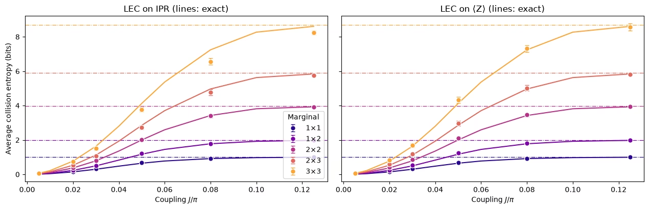
どちらの手法も被害の大部分を取り除きます。前のプロットの生の推定値はランダムすぎますが、緩和された推定値は厳密な曲線に沿っています。違いは、より大きな周辺分布で現れます。
小さな周辺分布では、どちらの手法もうまく機能します。 の周辺分布では、 に対するLECの方が明らかに近くなります。
IPRに対するLECでエントロピーが小さくなりすぎる理由。 エントロピーが小さすぎるということは、IPRが大きすぎるということです。IPRに対するLECはIPRを過剰に膨らませます。これは、ノイズがすべての のIPRへの寄与を同じ係数で減衰させると仮定しているためです。 では、すべての が に近いため、すべての文字列が等しく寄与し、ほとんどの文字列は中程度の重みを持ちます。 の周辺分布の511個の文字列のうち、252個は重み4または5で、重み1のものは9個しかありません。ノイズは重みが高い文字列ほど大きく減衰させるため(読み出しエラーだけでも、重み の文字列は で減衰します)、単一の係数 は主に中程度の重みの文字列の減衰によって決まります。 が大きくなると、重みの高い が最も速く減衰し、IPRはますます低重みの文字列によって担われるようになります。低重みの文字列はノイズによる減衰が小さいため、より強く減衰した文字列から主に学習した係数でそれらを増幅すると、IPRが過剰に膨らみます。周辺分布が大きいほど重みの範囲が広いため、この効果は周辺分布のサイズとともに大きくなります。また、文字列の構成が変化した後でも、IPRの一様値を超える分がまだ意味を持つ中間の で最大になります。
に対するLECが逆方向に誤る理由。 これは各文字列をそれぞれ固有の係数で再スケールするため、重み間のシフトの影響を受けません。仮定しているのは、各文字列が での減衰を保つということだけです。 が大きくなると、各 はより重みの高い演算子に広がり、それらは のときよりも多くのノイズを受けるため、係数は補正がわずかに不足し、エントロピーはわずかに高くなりすぎます。
したがって、ハードウェアで検証すべき予測は、周辺分布が大きいほど、 に対するLECが優位になるはずであるということです。ハードウェアではノイズはより強く、既知の形でもありません。
4. 大規模な実行
ハードウェア実験では、4サイクルの 格子を実行します。9つの結合で、48レイヤーに64量子ビットと1,344個のCZゲートがあります。シミュレーションと比べて、次の5点が変わります。
-
ノイズを学習する必要があり、これはCZレイヤーが固定されている場合にのみ機能します。
-
ツワーリングは、各レイヤーのノイズをパウリチャネルに変えます。これは学習も増幅もできます。
-
**動的デカップリング(DD)**がアイドル状態の量子ビットを保護します。
-
PEA用のノイズ増幅が、メインのデータと同じジョブで実行されます。
-
小さな でのMPSシミュレーションが、LECに基づくエラー緩和のための古典的な参照を提供します。
バックエンドが必要なセルは、RUN_ON_HARDWARE が True の場合にのみ実行されます。MPSシミュレーションは、COMPUTE_MPS_REFERENCES を True に設定すると再実行できます。その他のセルはここで実行されます。
# hardware run parameters:
num_cols_hw = num_rows_hw = 8
num_qubits_hw = num_cols_hw * num_rows_hw
num_cycles_hw = 4
couplings_hw = (
    np.array([0.005, 0.01, 0.02, 0.03, 0.05, 0.07, 0.09, 0.11, 0.125]) * np.pi
)
calibration_hw = 0  # J0 = 0.005π
disorder_hw = sample_disorder(
    num_cols_hw, num_rows_hw, np.random.default_rng(7)
)

# if running PEA:
noise_factors = np.array([1.0, 1.5, 2.0])  # PEA noise-amplification factors
固定CZレイヤー
def compile_by_sublayer(
    num_cols,
    num_rows,
    coupling,
    num_cycles,
    disorder,
    pass_manager,
    layout=None,
    num_physical_qubits=None,
):
    # Compile each sublayer once and repeat it with barriers, so the CZ layers are the
    # same in every cycle and at every coupling. The registers are named explicitly
    # because register names enter Samplomatic's box hashes. Bits land in lattice order.
    num_qubits = num_cols * num_rows
    if layout is None:
        layout, num_physical_qubits = list(range(num_qubits)), num_qubits
    blocks = []
    for sublayer in disorder:
        block = QuantumCircuit(num_qubits)
        for (i, j), (h_i, h_j) in sublayer:
            heisenberg_gate(block, coupling, i, j, h_i, h_j)
        blocks.append(pass_manager.run(block))
    circuit = QuantumCircuit(
        QuantumRegister(num_physical_qubits, "q"),
        ClassicalRegister(num_qubits, "meas"),
    )
    neel_state(circuit, num_cols, num_rows, layout)
    for _ in range(num_cycles):
        for block in blocks:
            circuit.compose(block, inplace=True)
            circuit.barrier(layout)
    circuit.measure(layout, range(num_qubits))
    return circuit
ノイズ学習のためのボックス
Samplomaticのボックス化パスマネージャーは、次に各回路をボックスにグループ化します。CZレイヤーごとに1つ、測定に1つです。各ボックスは必要なノイズモデルへの参照を持つため、すべての結合が同じボックスを共有していることを確認できます。次のセルは、バックエンドなしでCZゲートにコンパイルされた、ハードウェア実行の 回路に対してこれを行い、ノイズ学習が特性評価するボックスを出力します。
from samplomatic import build
from samplomatic.transpiler import generate_boxing_pass_manager
from samplomatic.utils import find_unique_box_instructions

boxing_pass_manager = generate_boxing_pass_manager(
    enable_gates=True,  # twirl the CZ layers
    enable_measures=True,  # twirl the measurements
    inject_noise_targets="gates",  # PEA amplifies the noise of the CZ layers only
    inject_noise_strategy="uniform_modification",
)

def noise_refs(boxed_circuit):
    return sorted(
        annotation.ref
        for box in find_unique_box_instructions(boxed_circuit.data)
        for annotation in box.operation.annotations
        if hasattr(annotation, "ref")
    )

# The 8x8 hardware circuits, compiled to CZ gates on the lattice qubits (no backend needed)
compiled_8x8 = [
    compile_by_sublayer(
        num_cols_hw, num_rows_hw, c, num_cycles_hw, disorder_hw, pass_manager
    )
    for c in couplings_hw
]
boxed_8x8 = [boxing_pass_manager.run(circuit) for circuit in compiled_8x8]
assert all(
    noise_refs(b) == noise_refs(boxed_8x8[0]) for b in boxed_8x8
), "layers differ between couplings"
num_cz, depth = two_qubit_stats(compiled_8x8[0])
print(
    f"{num_qubits_hw} qubits: {num_cz} CZ gates in {depth} layers, for every coupling"
)
for box in find_unique_box_instructions(boxed_8x8[0].data):
    ops = box.operation.blocks[0].count_ops()
    print(
        f"{box.operation.num_qubits}-qubit box: {ops.get('cz', 0)} CZ, {ops.get('measure', 0)} measurements"
    )
print(
    f"All {len(boxed_8x8)} couplings share these {len(find_unique_box_instructions(boxed_8x8[0].data))} boxes"
)
64 qubits: 1344 CZ gates in 48 layers, for every coupling
64-qubit box: 32 CZ, 0 measurements
64-qubit box: 24 CZ, 0 measurements
64-qubit box: 32 CZ, 0 measurements
64-qubit box: 24 CZ, 0 measurements
64-qubit box: 0 CZ, 64 measurements
All 9 couplings share these 5 boxes
回路をツワーリングする
ランダム化のたびに、Samplomaticは各ボックスの前にランダムなパウリゲートを、後ろにそれを補償するゲートを置き、隣接する1量子ビット・ゲートにマージします。ランダム化にわたって平均すると、各レイヤーのノイズはパウリチャネルになり、NoiseLearnerV3 はこれをスパース・パウリ・リンドブラッド・モデルとして学習でき、PECステップではなくPEAステップがこれを増幅できます。測定のツワーリングでは、読み出しの前にビットをランダムに反転します。反転はソフトウェアで元に戻され、これにより読み出しノイズが対称になり、読み出し補正(TREX)の基礎となります。
ハードウェアのワークフロー
量子ビットを選び、回路をコンパイルし、ノイズを学習してスイープを実行します。これらのセルはここではオフになっています。
量子ビットを選ぶ。 Nighthawkの正方グリッドは、SWAPゲートなしで 格子を収容します。このセルは、グリッドのすべての 矩形を、報告されたCZエラーと読み出しエラーでスコア付けし、最良のものを選びます。
def square_layouts(backend, side):
    # Every side x side rectangle of the square qubit grid that supports all bonds
    target = backend.target

    def has_cz(a, b):
        return (a, b) in target["cz"] or (b, a) in target["cz"]

    stride = next(
        s
        for s in (10, 12)
        if all(has_cz(q, q + s) for q in range(backend.num_qubits - s))
    )
    layouts = []
    for y0 in range(backend.num_qubits // stride - side + 1):
        for x0 in range(stride - side + 1):
            layout = [
                stride * (y0 + y) + x0 + x
                for y in range(side)
                for x in range(side)
            ]
            bonds = [
                bond
                for layer in brickwork_layers(side, side)
                for bond in layer
            ]
            if all(has_cz(layout[i], layout[j]) for i, j in bonds):
                layouts.append(((x0, y0), layout))
    return layouts

def layout_score(backend, layout, side, uses_per_bond):
    # Minus the summed log-fidelity of the bonds (each used uses_per_bond times) and readouts
    properties, target = backend.properties(), backend.target
    cz_errors = []
    for i, j in (
        bond for layer in brickwork_layers(side, side) for bond in layer
    ):
        pair = (
            (layout[i], layout[j])
            if (layout[i], layout[j]) in target["cz"]
            else (layout[j], layout[i])
        )
        cz_errors.append(properties.gate_error("cz", pair))
    readout_errors = [properties.readout_error(q) for q in layout]
    if max(cz_errors) >= 0.5 or max(readout_errors) >= 0.25:
        return np.inf  # an unusable qubit or bond
    return float(
        -uses_per_bond * np.log1p(-np.array(cz_errors)).sum()
        - np.log1p(-np.array(readout_errors)).sum()
    )

if RUN_ON_HARDWARE:
    from qiskit_ibm_runtime import QiskitRuntimeService

    def holds_lattice(backend):
        try:
            return bool(square_layouts(backend, num_cols_hw))
        except (KeyError, StopIteration):
            return False

    service = QiskitRuntimeService()
    candidates = [
        b
        for b in service.backends(operational=True, simulator=False)
        if holds_lattice(b)
    ]
    backend = min(candidates, key=lambda b: b.status().pending_jobs)
    score, origin, initial_layout = min(
        (
            layout_score(backend, layout, num_cols_hw, 3 * num_cycles_hw),
            origin,
            layout,
        )
        for origin, layout in square_layouts(backend, num_cols_hw)
    )
    print(f"{backend.name}: origin {origin}, score {score:.2f}")
コンパイル。 選んだ量子ビット上で上記と同じ手順を行い、続いて build を実行します。これは、各ボックス化された回路をテンプレート回路とsamplex(ツワーリングゲートと注入されるノイズを引き出すためのレシピ)に変換します。DDはテンプレートに追加されます。
if RUN_ON_HARDWARE:
    from qiskit_ibm_runtime.executor.dynamical_decoupling import (
        generate_dd_pass_manager,
    )
    from qiskit_ibm_runtime.options import DynamicalDecouplingOptions

    # PEA structure functions:
    target_pass_manager = generate_preset_pass_manager(
        target=backend.target,
        optimization_level=3,
        initial_layout=initial_layout,
        routing_method="none",
        seed_transpiler=7,
    )
    boxed_hw = [
        boxing_pass_manager.run(
            compile_by_sublayer(
                num_cols_hw,
                num_rows_hw,
                coupling,
                num_cycles_hw,
                disorder_hw,
                target_pass_manager,
                layout=initial_layout,
                num_physical_qubits=backend.num_qubits,
            )
        )
        for coupling in couplings_hw
    ]
    assert all(noise_refs(b) == noise_refs(boxed_hw[0]) for b in boxed_hw)
    unique_boxes_hw = find_unique_box_instructions(boxed_hw[0].data)

    # DD pass:
    dd_pass_manager = generate_dd_pass_manager(
        backend,
        DynamicalDecouplingOptions(
            enable=True,
            sequence_type="XY4",
            scheduling_method="alap",
            extra_slack_distribution="middle",
            skip_reset_qubits=False,
        ),
    )
    templates = []
    for circuit in boxed_hw:
        template, samplex = build(circuit)
        templates.append((dd_pass_manager.run(template), samplex))
ノイズを学習してスイープを実行する。 1つの NoiseLearnerV3 ジョブが5つのボックスすべてを学習します。4つのCZレイヤーそれぞれのパウリ・リンドブラッド・モデルと、測定ボックスの読み出しノイズです。次に、1つの QuantumProgram が9つの結合すべてを保持します。各アイテムには、テンプレート、samplex、学習済みのノイズモデル、3つのノイズスケールが与えられます。スケール0は、両方のLEC手法のための増幅されていないデータです。スケール0.5と1は、PEAのために学習したノイズの50%と100%を加え、PEAはゼロノイズへ外挿します。これには約40秒のQPU時間を使用します。
if RUN_ON_HARDWARE:
    from qiskit_ibm_runtime import Executor, NoiseLearnerV3, QuantumProgram

    # Learn the noise of the five boxes
    learner = NoiseLearnerV3(backend)
    learner.options.num_randomizations = 32
    learner.options.shots_per_randomization = 128
    # Up to 24 layer pairs, the depth of the 48-layer circuits
    learner.options.layer_pair_depths = [0, 1, 2, 4, 16, 24]
    learner_job = learner.run(unique_boxes_hw)
    print("Noise learning job:", learner_job.job_id())

    # Run the sweep, with the learned noise amplified by each of the noise factors
    noise_maps = learner_job.result().to_dict(
        instructions=unique_boxes_hw, require_refs=False
    )
    program = QuantumProgram(shots=200)
    for template, samplex in templates:
        program.append_samplex_item(
            template,
            samplex=samplex,
            samplex_arguments={
                "pauli_lindblad_maps": noise_maps,
                **{
                    f"noise_scales.{ref}": (noise_factors - 1).reshape(-1, 1)
                    for ref in noise_maps
                },
            },
            shape=(len(noise_factors), 200),  # noise scales x randomizations
        )
    executor_job = Executor(backend).run(program)
    print("Executor job:", executor_job.job_id())
    # Section 5 converts the results of these two jobs and saves them
5. ハードウェアのデータ
このセクションでは、これまでの手法がNighthawkプロセッサの実際のハードウェアデータでどのように機能するかを調べます。
実行を読み込む
RUN_ON_HARDWARE を True に設定すると、次のセルはセクション4の2つのジョブの結果を変換し、保存済みの実行と同じ形式で data/hardware_run_new.npz に保存します。これにより、新しい実行を後で再び解析できます。そうでない場合は、data/hardware_run.npz から保存済みの実行を読み込みます。ビットは、スペースを節約するために量子ビット軸に沿ってパックされています。
ジョブの実行中にカーネルが再起動した場合は、ジョブを再送信しないでください。セクション4の最後の呼び出しより前のセルを再実行し、同じ量子ビットが選ばれることを確認して、セクション4で出力されたジョブIDを使い、learner_job と executor_job を service.job(job_id) に設定してください。
if RUN_ON_HARDWARE:

    def unflip(item_result):
        # Undo the measurement twirling of an Executor item: flip back the bits that were flipped
        return item_result["meas"] ^ item_result["measurement_flips.meas"]

    learner_result = learner_job.result()
    raw_bits = [unflip(item) for item in executor_job.result()]

    # The learned readout map indexes the measured qubits in ascending physical order;
    # relabel it to lattice order
    measurement_box_index = next(
        k
        for k, box in enumerate(unique_boxes_hw)
        if "measure" in box.operation.blocks[0].count_ops()
    )
    measurement_box = next(
        inst
        for inst in boxed_hw[0].data
        if inst.operation.name == "box"
        and "measure" in inst.operation.blocks[0].count_ops()
    )
    measured = sorted(
        boxed_hw[0].find_bit(q).index for q in measurement_box.qubits
    )
    lattice_index = {physical: q for q, physical in enumerate(initial_layout)}
    readout_map = (
        learner_result[measurement_box_index]
        .to_pauli_lindblad_map()
        .apply_layout([lattice_index[p] for p in measured], num_qubits_hw)
    )

    # Save the run in the same format as the saved run, so it can be analyzed again later
    terms = readout_map.to_sparse_list()
    np.savez_compressed(
        "data/hardware_run_new.npz",
        bits=np.packbits(np.stack(raw_bits), axis=-1, bitorder="little"),
        labels=np.array([label for label, _, _ in terms]),
        indices=np.concatenate(
            [np.asarray(support) for _, support, _ in terms]
        ),
        rates=np.array([rate for _, _, rate in terms]),
        physical_qubits=np.array(initial_layout),
        couplings_over_pi=couplings_hw / np.pi,
        noise_factors=noise_factors,
    )
else:
    saved = np.load(
        "data/hardware_run.npz"
    )  # or data/hardware_run_new.npz, for a new run
    raw_bits = list(
        np.unpackbits(
            saved["bits"], axis=-1, count=num_qubits_hw, bitorder="little"
        ).astype(bool)
    )
    labels = [str(label) for label in saved["labels"]]
    indices = np.split(
        saved["indices"], np.cumsum([len(label) for label in labels])[:-1]
    )
    readout_map = PauliLindbladMap.from_sparse_list(
        list(zip(labels, indices, saved["rates"])), num_qubits_hw
    )

print(f"{len(raw_bits)} couplings, bits per coupling: {raw_bits[0].shape}")
print(
    f"Readout noise: {readout_map.num_terms} terms on {readout_map.num_qubits} qubits"
)
9 couplings, bits per coupling: (3, 200, 200, 64)
Readout noise: 64 terms on 64 qubits
古典的な参照
どちらのLEC手法も、 での理想的な周辺分布を必要とし、それらをテストするには、保留した結合 と での理想値が必要です。これらは行列積状態(MPS)シミュレーションから得られ、論文と同様に、各周辺分布の形状の格子上のすべての配置について、また ではすべての重ならない ブロックについて保存されています。 では、ボンド次元 で収束します。 と では を使用しており、 では の周辺分布で から最大約13%まだ変化するため、そこでは近似値として扱ってください。次のセルは、COMPUTE_MPS_REFERENCES が True の場合はこれらを計算し(約18分かかります)、そうでない場合は、結合のインデックス、ボンド次元、周辺分布をキーとして保存された結果を読み込みます。
# Every placement of every shape on the 8x8 lattice
positions = {
    label: all_positions(shape, num_cols_hw, num_rows_hw)
    for label, shape in patch_shapes.items()
}
reference_settings = [
    (calibration_hw, 32),
    (calibration_hw, 64),
    (1, 128),
    (2, 64),
    (2, 128),
]  # (coupling, χ)

if COMPUTE_MPS_REFERENCES:

    def mps_patch_probabilities(coupling, patches, bond_dimension):
        # Distributions of the given marginals after the 8x8 circuit, from an MPS simulation
        simulator = AerSimulator(
            method="matrix_product_state",
            matrix_product_state_max_bond_dimension=bond_dimension,
            matrix_product_state_truncation_threshold=1e-12,
        )
        circuit = heisenberg_floquet_circuit(
            num_cols_hw,
            num_rows_hw,
            coupling,
            num_cycles_hw,
            disorder_hw,
            measure=False,
        )
        circuit = generate_preset_pass_manager(
            optimization_level=1, basis_gates=["cx", "u"], seed_transpiler=7
        ).run(circuit)
        for label, qubits in patches.items():
            circuit.save_probabilities(qubits, label=label)
        data = simulator.run(circuit, shots=1).result().data(0)
        return {label: np.asarray(data[label]) for label in patches}

    placements = {
        f"{label} {k}": qubits
        for label, patch_list in positions.items()
        for k, qubits in enumerate(patch_list)
    }
    tiles = {
        f"site {q}": [q] for q in range(num_qubits_hw)
    } | {  # for the lattice map at J0
        f"block {x},{y}": patch_qubits((2 * x, 2 * y), (2, 2), num_cols_hw)
        for y in range(num_rows_hw // 2)
        for x in range(num_cols_hw // 2)
    }
    computed = {}
    for index, chi in reference_settings:
        targets = (
            placements | tiles
            if (index, chi) == (calibration_hw, 64)
            else placements
        )
        for key, p in mps_patch_probabilities(
            couplings_hw[index], targets, chi
        ).items():
            computed[f"{index}/{chi}/{key}"] = p
    np.savez_compressed("data/mps_references_all.npz", **computed)
    saved = computed
else:
    saved = np.load("data/mps_references_all.npz")

references = {}  # (coupling index, bond dimension) -> {marginal key: distribution}
for name in saved:
    index, chi, key = name.split("/", 2)
    references.setdefault((int(index), int(chi)), {})[key] = saved[name]
データ品質: 不良なカプラー/量子ビット
まず、最も小さい結合 を見てみましょう。ここでは期待値がネールのチェッカーボードに近いはずです。
# <Z> of every site at J0: the MPS reference, and the hardware data at noise factor 1
z_reference = np.array(
    [
        parities_from_probabilities(
            references[(calibration_hw, 64)][f"site {q}"]
        )[0]
        for q in range(num_qubits_hw)
    ]
)
z_measured = 1 - 2 * raw_bits[calibration_hw][0].mean(axis=(0, 1))
fig, axes = plt.subplots(1, 2, figsize=(11, 4.6), layout="constrained")
fig.get_layout_engine().set(wspace=0.12)  # white space between the two panels
edges = np.arange(num_cols_hw + 1) - 0.5
for ax, values, title in zip(
    axes, (z_reference, z_measured), ("MPS reference", "Hardware")
):
    mesh = ax.pcolormesh(
        edges,
        edges,
        values.reshape(num_rows_hw, num_cols_hw),
        cmap="RdBu_r",
        vmin=-1,
        vmax=1,
        edgecolors="white",
    )
    ax.set_aspect("equal")
    ax.invert_yaxis()
    ax.set_xticks([])
    ax.set_yticks([])
    ax.set_title(
        f"{title}, $J_0 = {couplings_hw[calibration_hw] / np.pi:g}\\pi$"
    )
fig.colorbar(
    mesh, ax=axes, shrink=0.8, label=r"$\langle Z \rangle$ of each site"
)
plt.show()

Question. ハードウェアマップを見て、何が目を引きますか?
答え
淡い色のサイトです。 での状態はネール状態に近いにもかかわらず、信号をほとんど失っています。LECは で残っている信号で割り算を行うため、これらは重要です。信号がほとんどない量子ビットは、巨大でノイズの多い補正係数を生み、そのような量子ビットが少数あるだけで、それを含むすべての周辺分布を支配しかねません。
データだけを使うルール: での1量子ビットIPRが、完全に混合した量子ビットの値である から 以内にある場合、その量子ビットは不良です。1量子ビットのIPRは なので、これにより の量子ビットにフラグが立ちます。フラグが立ったサイトを含む周辺分布は、以下では除外されます。
site_iprs = np.array(
    [
        ipr_from_shots(raw_bits[calibration_hw][0][:, :, [q]])
        for q in range(num_qubits_hw)
    ]
)
# |IPR - 1/2| < 0.25**2 / 2 is the same as |<Z>| < 0.25
flagged = {
    q for q in range(num_qubits_hw) if abs(site_iprs[q] - 0.5) < 0.25**2 / 2
}
print(
    f"Median single-qubit IPR at J0: {np.median(site_iprs):.2f}; flagged lattice sites {sorted(flagged)}"
)
Median single-qubit IPR at J0: 0.77; flagged lattice sites [19, 24, 25, 27, 32]
平均する周辺分布を選択する
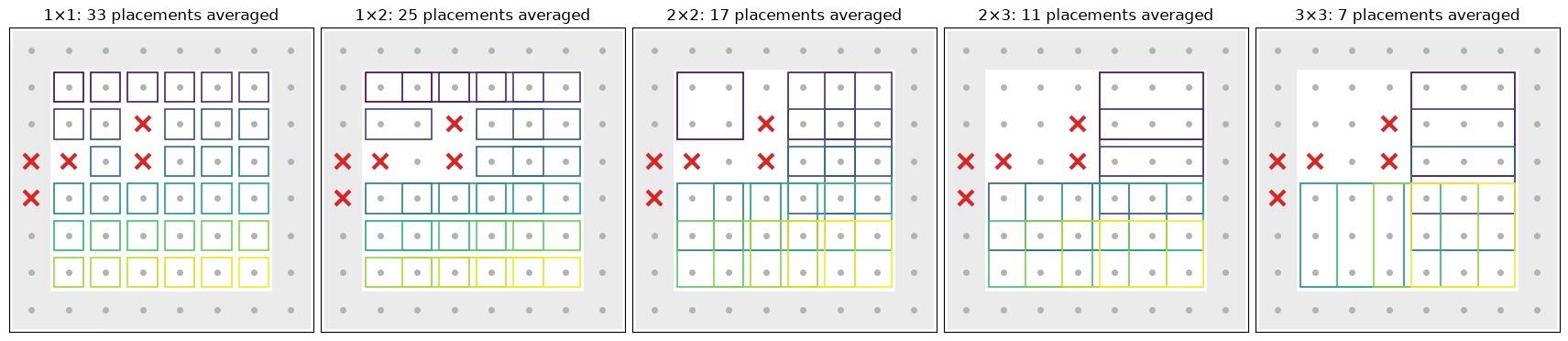
次のセルは、以下の平均に含まれる各形状の配置を示します。フラグが立てられたサイト(赤い十字)のない格子のバルク部分にあるすべての配置です。端に接する配置(網掛け)は除外されます。端の量子ビットは結合が少ないため、スクランブルがより遅くなります。それらだけで平均すると、すべての形状と手法で、バルクの配置より の1ステップ分だけ遅れて交差します。平均した各配置にはそれぞれのボックスがあり、配置ごとに色分けされています。
def touches_edge(qubits):
    # Whether a placement includes a site on the edge of the lattice
    return any(
        q % num_cols_hw in (0, num_cols_hw - 1)
        or q // num_cols_hw in (0, num_rows_hw - 1)
        for q in qubits
    )

# The placements of each shape that enter the averages: in the bulk, and without a flagged site
kept_placements = {
    label: [
        k
        for k, qubits in enumerate(patch_list)
        if not touches_edge(qubits) and not set(qubits) & flagged
    ]
    for label, patch_list in positions.items()
}
placement_cmap = plt.get_cmap("viridis")
fig, axes = plt.subplots(
    1, len(positions), figsize=(17, 4.4), layout="constrained"
)
for ax, (label, patch_list) in zip(axes, positions.items()):
    width, height = patch_shapes[label]
    for q in range(num_qubits_hw):
        x, y = q % num_cols_hw, q // num_cols_hw
        if touches_edge([q]):  # shade the edge of the lattice
            ax.add_patch(
                plt.Rectangle(
                    (x - 0.5, y - 0.5), 1, 1, color="0.92", zorder=0
                )
            )
        ax.plot(x, y, "o", color="0.7", ms=4, zorder=1)
    kept = kept_placements[label]
    for i, k in enumerate(kept):
        qubits = patch_list[k]
        x0, y0 = (
            qubits[0] % num_cols_hw,
            qubits[0] // num_cols_hw,
        )  # top-left site of the placement
        ax.add_patch(
            plt.Rectangle(
                (x0 - 0.4, y0 - 0.4),
                width - 0.2,
                height - 0.2,
                fill=False,
                lw=1.2,
                ec=placement_cmap(i / max(len(kept) - 1, 1)),
                zorder=2,
            )
        )
    for q in flagged:
        ax.plot(
            q % num_cols_hw,
            q // num_cols_hw,
            "x",
            color="#d62728",
            ms=11,
            mew=3,
            zorder=3,
        )
    ax.set_xlim(-0.6, num_cols_hw - 0.4)
    ax.set_ylim(num_rows_hw - 0.4, -0.6)
    ax.set_aspect("equal")
    ax.set_xticks([])
    ax.set_yticks([])
    ax.set_title(f"{label}: {len(kept)} placements averaged")
plt.show()
PEA
3つ目の手法は、古典的な参照を必要としません。各パリティについて、ノイズ係数 1、1.5、2 の値を取り、学習した読み出し減衰(TREX)で割り、ノイズ係数に対する指数関数をフィットして、ゼロノイズへ外挿します。符号が変わるパリティやほぼゼロのパリティには、直線フィットを使います。分散を差し引くには、その信頼できる推定値が必要です。これは生のパリティや再スケールしたパリティでは簡単ですが、クリッピングやフォールバックを伴う非線形フィットの出力では簡単ではありません。そのため PEA は、2乗のバイアスを除去するもう1つの標準的な方法を使います。ランダム化の半分ずつを別々に外挿し、2つの独立した推定値を掛け合わせます。
def readout_fidelity(support):
    # Damping of <Z_S> by the learned readout noise
    pauli = QubitSparsePauli.from_sparse_label(
        ("Z" * len(support), list(support)), num_qubits_hw
    )
    return readout_map.pauli_fidelity(pauli)

def extrapolate_to_zero(values):
    # Fit a * exp(b * factor) to each column of values (noise factors first), or a line
    # where the values change sign or come within 1e-3 of zero
    result = np.polynomial.polynomial.polyfit(noise_factors, values, 1)[0]
    sign = np.sign(values[0])
    usable = np.all(np.sign(values) == sign, axis=0) & (
        np.abs(values).min(axis=0) > 1e-3
    )
    if usable.any():
        log_fit = np.polynomial.polynomial.polyfit(
            noise_factors, np.log(np.abs(values[:, usable])), 1
        )
        result[usable] = sign[usable] * np.exp(log_fit[0])
    return result

def pea_ipr(parities, fidelities, num_patch):
    # parities has shape (noise factors, randomizations, supports). Extrapolate the two
    # halves of the randomizations separately; their errors are independent, so the
    # product of the two estimates of each parity has no shot-noise bias
    def zero_noise(p):
        # A parity cannot exceed 1 in magnitude, so cap the extrapolated values there
        return np.clip(
            extrapolate_to_zero(p.mean(axis=1) / fidelities), -1, 1
        )

    half = parities.shape[1] // 2
    first, second = (
        zero_noise(parities[:, :half]),
        zero_noise(parities[:, half:]),
    )
    return float((1 + np.dot(first, second)) / 2**num_patch)
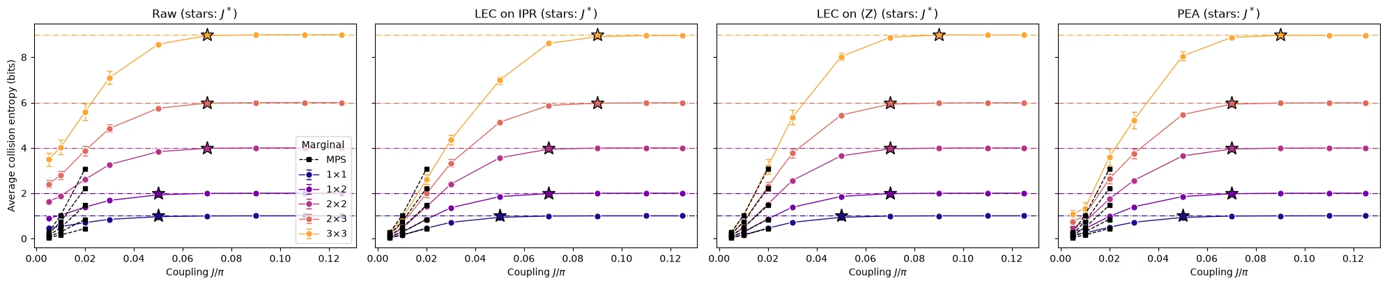
4つの推定値すべてと交差点
次の関数は、すべての結合について、1つの周辺分布位置の IPR に対する、生の推定値、IPR 上の LEC、 上の LEC、PEA の推定値を計算します。また、ランダム化をブートストラップすることで、それぞれのショットノイズも推定します。このセルは、平均に含まれるすべての配置に対してこれを実行し、約1分半かかります。
def estimate_iprs(qubits, key):
    # Raw, LEC-on-IPR, LEC-on-<Z>, and PEA IPRs of one marginal position at every coupling,
    # with the shot noise of each from a bootstrap over the randomizations
    n = len(qubits)
    supports = parity_supports(qubits)
    # Parities with shape (noise factors, randomizations, supports), per coupling
    parities = [
        np.stack([parity_expectation_values(b, supports) for b in bits])
        for bits in raw_bits
    ]
    patch_bits = [
        bits[0][:, :, qubits] for bits in raw_bits
    ]  # noise factor 1
    values, errors = lec_estimates(
        patch_bits,
        [p[0] for p in parities],
        references[(calibration_hw, 64)][key],
        calibration_hw,
        n,
    )
    fidelities = np.array([readout_fidelity(s) for s in supports])

    def pea_statistic(p):
        return pea_ipr(p, fidelities, n)

    values["raw"] = [ipr_from_shots(b) for b in patch_bits]
    errors["raw"] = [bootstrap_error(ipr_from_shots, b) for b in patch_bits]
    values["PEA"] = [pea_statistic(p) for p in parities]
    errors["PEA"] = [
        bootstrap_error(pea_statistic, p, axis=1) for p in parities
    ]  # randomizations are axis 1
    return {m: np.array(v) for m, v in values.items()}, {
        m: np.array(e) for m, e in errors.items()
    }

methods = ["LEC on IPR", "LEC on ⟨Z⟩", "PEA"]
method_colors = {
    "LEC on IPR": "#2a78d6",
    "LEC on ⟨Z⟩": "#1baf7a",
    "PEA": "#eb6834",
}
iprs, ipr_errors = {}, {}
for label, patch_list in positions.items():
    for k in kept_placements[label]:
        iprs[label, k], ipr_errors[label, k] = estimate_iprs(
            patch_list[k], f"{label} {k}"
        )
print(f"{len(iprs)} clean marginal positions")
93 clean marginal positions
def crossover_coupling(couplings, entropies, haar, tolerance=0.1):
    # Smallest coupling whose entropy is within tolerance of the random-state value
    for coupling, entropy in zip(couplings, entropies):
        if entropy >= haar - tolerance:
            return coupling
    return None

def reference_ipr(index, chi, key):
    # IPR of the MPS distribution of a marginal
    return float((references[(index, chi)][key] ** 2).sum())

mps_settings = [
    (calibration_hw, 64),
    (1, 128),
    (2, 128),
]  # (coupling index, bond dimension)
panels = ["raw", *methods]

# Average IPR of every shape over its clean placements, then the entropy and the crossover
hw_entropies = {
    method: {} for method in panels
}  # per method and shape: average entropy and its error
crossovers = {method: {} for method in panels}
mps_entropies = {}  # per shape: MPS entropy, averaged over the same placements, at mps_settings
for label, patch_list in positions.items():
    haar = haar_entropy(len(patch_list[0]), num_qubits_hw)
    keys = [(shape, k) for (shape, k) in iprs if shape == label]
    mps_entropies[label] = [
        collision_entropy(
            np.mean([reference_ipr(j, chi, f"{label} {k}") for _, k in keys])
        )
        for j, chi in mps_settings
    ]
    for method in panels:
        ipr, ipr_error = average_ipr(
            [iprs[key][method] for key in keys],
            [ipr_errors[key][method] for key in keys],
        )
        entropy = collision_entropy(ipr)
        hw_entropies[method][label] = (entropy, ipr_error / (ipr * np.log(2)))
        crossovers[method][label] = crossover_coupling(
            couplings_hw, entropy, haar
        )
fig, axes = plt.subplots(
    1, len(panels), figsize=(5 * len(panels), 4.2), sharey=True
)
for (label, patch_list), color in zip(positions.items(), colors):
    haar = haar_entropy(len(patch_list[0]), num_qubits_hw)
    for ax, method in zip(axes, panels):
        entropy, error = hw_entropies[method][label]
        ax.errorbar(
            couplings_hw / np.pi,
            entropy,
            yerr=error,
            fmt="o-",
            color=color,
            mec="white",
            ms=7,
            lw=1,
            capsize=3,
            label=label,
        )
        ax.plot(
            couplings_hw[[j for j, _ in mps_settings]] / np.pi,
            mps_entropies[label],
            "s--",
            color="black",
            ms=4,
            lw=1,
            label="MPS" if label == "3×3" else None,
            zorder=4,
        )
        ax.axhline(haar, color=color, ls="dashdot", lw=0.9)
        if crossovers[method][label]:
            ax.plot(
                crossovers[method][label] / np.pi,
                haar,
                "*",
                ms=14,
                color=color,
                mec="black",
                zorder=3,
            )
for ax, method in zip(axes, panels):
    ax.set_title(f"{'Raw' if method == 'raw' else method} (stars: $J^*$)")
    ax.set_xlabel("Coupling $J/\\pi$")
axes[0].set_ylabel("Average collision entropy (bits)")
axes[0].legend(title="Marginal", loc="lower right")
fig.tight_layout()
plt.show()
まとめ
この規模の実験を実行するために必要だったこと:
-
構造が に依存しない回路。1サブレイヤーずつコンパイルするため、1つのノイズモデルでスイープ全体に対応できます。
-
ビット列から計算する推定量。周辺分布の IPR にはペアカウント、緩和された期待値が入力の場合には、各2乗パリティから分散を差し引くパーセバル形式を使います。
-
安価な古典的アンカー。小さな での理想状態でノイズを較正し、保持した結合でその較正をテストします。IPR 全体ではなく各 を個別に較正することで、大きな周辺分布が一致するようになります。
-
重い処理のための IBM ツール。Samplomatic のボックスとツワーリング、
NoiseLearnerV3、動的デカップリング、そして PEA のためのノイズ増幅を伴う1つのExecutorジョブ。 -
データのみを使用するデータ品質チェック。
次のステップ。 エラー緩和をさらに進めるには、probabilistic error amplification と PEC with shaded lightcones のチュートリアルを参照してください。