AQC + Trotterダイナミクス・サーバーレス・ワークフローで中性子散乱をシミュレートする

使用量の見積もり: Heron r3プロセッサで18分(注: これはあくまで見積もりです。実際の実行時間は異なる場合があります。)

学習成果

• 非弾性中性子散乱スペクトルが1次元量子磁性体の動的構造因子$S(q, \omega)$にどのようにマッピングされるか。

• 密度行列繰り込み群(DMRG)と行列積状態(MPS)忠実度最大化を用いてKCuF$_3$(等方性ハイゼンベルク)基底状態を準備する方法。

• Trotter時間発展、近似量子コンパイル(AQC)回路圧縮、および誤り軽減付き実行を単一の関数呼び出しとして実行する方法。

• サイトごとの$\langle \sigma_z \rangle(t)$時系列を後処理して$S(q, \omega)$にし、2スピノン連続体を特定する方法。

前提条件

• Qiskitパターン、SparsePauliOp、およびTrotter時間発展に精通していること。

• テンソル・ネットワーク法(DMRGとMPS)への基本的な理解があると役立ちますが必須ではありません。同様に、関数がTrotter回路を圧縮するために使用するqiskit-addon-aqc-tensorライブラリへの精通も必須ではありません。

背景

非弾性中性子散乱は、スピン-スピン相関関数の空間・時間フーリエ変換である動的構造因子$S(q, \omega)$を測定するため、微視的スピン・モデルから$S(q, \omega)$を再現することは、量子シミュレーションの直接的で反証可能なテストとなります。このチュートリアルでは、KCuF$_3$を研究します。これはスピン-$\frac{1}{2}$反強磁性ハイゼンベルク鎖であり、その励起は単一のスピン反転ではなく、フラクショナル化したスピノンのペアです。鋭いマグノン分散の代わりに、$S(q, \omega)$は広い2スピノン連続体を示し、下は$\tfrac{\pi}{2}|\sin q|$、上は$\pi|\sin(q/2)|$で境界づけられています。これらは、以下のプロットに表示される破線曲線です。物理の全容と、測定された中性子データとの比較は、元のチュートリアルおよびLeeら, arXiv:2603.15608で扱われています。

量子ワークフローは散乱実験を反映しています。

1. 鎖の基底状態$|\psi_0\rangle$を準備する。

2. 中心サイトで局所的な摂動($\pi/2$の$Z$回転)を加え、中性子からの運動量とエネルギーの移動を模倣する。

3. Trotter積公式を用いて、ハイゼンベルク・ハミルトニアン$e^{-iHt}$の下で時間発展させる。

4. サイトごとの磁化$\langle \sigma_z^j \rangle(t)$を測定する。サイト$j$と時間$t$の関数として、これはまさに遅延グリーン関数$G^R(j, j_c, t)$であるため、ステップ5でのフーリエ変換の前に変換は必要ありません。

5. $G^R$をフーリエ変換して$S(q, \omega)$にする。

問題はステップ3で発生する可能性があります。長時間の発展に対する厳密なTrotter回路がハードウェアには深すぎる場合です。テンソル・ネットワークを用いたAQCは、Trotterステップのブロックを、MPSシミュレータを用いて古典的に厳密な発展への状態忠実度が最大化される、固定された浅いパラメータ化アンザッツに圧縮することでこれに対処します(arXiv:2301.08609)。AQCダイナミクス・テンプレートは、この量子コア全体(Trotter合成、AQC圧縮、および誤り軽減付き実行)を1回の呼び出しにパッケージ化しています。

前処理(このノートブック)	関数(aqc-dynamics-function)	後処理(このノートブック)
DMRGとMPS忠実度最大化による基底状態。中性子キックは同じ回路に組み込まれる	Trotter合成 → AQC圧縮 → statevector、fake、またはruntime上での実行。サイトごとの$\langle \sigma_z^j \rangle(t)$を返す	$S(q, \omega)$、動的構造因子

実験に固有の作業は、このノートブック内に留まります。基底状態の準備(前処理)と$S(q, \omega)$の後処理(後処理)です。量子計算負荷の高い2つのステップ、圧縮と実行は、関数内で実行されます。

このチュートリアルは、量子回路を用いた量子材料での中性子散乱のシミュレーションの姉妹編であり、そちらでは同じ実験をインラインで構築しています。同じKCuF$_3$モデル、基底状態の準備、中性子キック、そして後処理を、Trotter合成、AQC圧縮、誤り軽減付き実行をステップごとに書き出して行っています。AQC圧縮の仕組みを学ぶにはそのチュートリアルを読んでください。デプロイされた関数テンプレートを通じて同じ実験を実行するにはこちらを読んでください。量子コアは単一の関数呼び出しになり、数時間かかるAQC圧縮はお使いのマシン上ではなくサーバーレス・ワーカー内で実行されるため、実行中にHPCシステムやオープンなカーネルは必要ありません。同じ呼び出しは、他の1次元ダイナミクス実験も駆動します。

要件

このチュートリアルを開始する前に、以下を用意してください。

• Qiskit Serverlessアカウントにデプロイされた関数。まず姉妹編である関数テンプレートを実行してください: AQC + Trotterダイナミクス関数テンプレートのデプロイと実行。そのガイドでは、ソースファイルの入手方法とアカウントへの関数のアップロード方法を説明しています。このチュートリアルは、デプロイされた関数を呼び出すだけです。

• QiskitServerless用に保存されたIBM Quantum®の認証情報(関数テンプレートを参照)。このチュートリアルの両方の例がデプロイされた関数を呼び出すため、両方ともこれが必要です。

• Qiskit SDK v2.0以降(pip install qiskit)。

• Qiskit IBM Catalogクライアント(pip install qiskit-ibm-catalog)。

• NumPy、SciPy、Matplotlib(pip install numpy scipy matplotlib)。基底状態の準備で使用するCOBYQAオプティマイザーには、SciPy 1.14以降が必要です。

• AQCテンソル・ネットワーク・スタック。ステップ1の基底状態の準備は、このノートブック内でローカルに実行されるため必要です: pip install 'qiskit-addon-aqc-tensor[quimb-jax]==0.3.1'。

新しくデプロイされた関数への最初の呼び出しは、サーバーレス・ワーカーが依存関係をインストールする間待機するため、その実行では追加のレイテンシが予想されます。

セットアップ

ライブラリをインポートし、後で使用する実験固有のヘルパーを定義します: build_gs_ansatz(基底状態準備のためのハミルトニアン変分アンザッツ、HVA)、prepare_ground_state(DMRGとMPS忠実度最大化)、そしてget_spectrum、plot_green、plot_spectrum($S(q, \omega)$の後処理)。これらは元の中性子散乱チュートリアルから適応されています。

# Added by doQumentation — required packages for this notebook
!pip install -q matplotlib numpy qiskit qiskit-addon-aqc-tensor qiskit-ibm-catalog quimb scipy

from functools import partial

import matplotlib.pyplot as plt
import numpy as np
import scipy.optimize

import quimb.tensor as qtn
from qiskit import QuantumCircuit
from qiskit.quantum_info import SparsePauliOp
from qiskit_addon_aqc_tensor.simulation import tensornetwork_from_circuit
from qiskit_addon_aqc_tensor.simulation.quimb import QuimbSimulator
from qiskit_ibm_catalog import QiskitServerless

#  Dynamical structure factor via discrete Fourier transform

def get_spectrum(n, Gjjc, dt, time_steps, q_steps, w_steps):
    """Compute the dynamical structure factor from the retarded Green's function.

    Uses the center-site approximation and a discrete Fourier transform.
    """
    green = Gjjc / 4  # sigma -> S=1/2
    omega_max = np.pi / dt
    qpoints = np.arange(0, 2 * np.pi, 2 * np.pi / q_steps)
    omegas = np.arange(0, omega_max, omega_max / w_steps)
    green_map = np.zeros((omegas.shape[0], qpoints.shape[0]))
    center = n // 2 - 1
    for iw, w in enumerate(omegas):
        exponent = np.exp(1j * w * dt * np.arange(1, time_steps + 1))
        S_w = np.dot(green.T, exponent) * dt
        for iq, q in enumerate(qpoints):
            q_matrix = np.exp(-1j * q * np.arange(-center, center + 2, 1))
            green_map[iw, iq] = np.imag(np.dot(S_w, q_matrix))
    return green_map

#  Plotting helpers

def plot_spectrum(
    dsf,
    dt,
    q_steps,
    w_steps,
    lower_bound=False,
    upper_bound=False,
    title=None,
):
    """Heat-map of the dynamical structure factor."""
    omega_max = np.pi / dt
    qpoints = np.arange(0, 2 * np.pi, 2 * np.pi / q_steps)
    omegas = np.arange(0, omega_max, omega_max / w_steps)
    x, y = np.meshgrid(qpoints, omegas)
    fig, ax = plt.subplots(figsize=(8, 5))
    c = ax.pcolormesh(x, y, dsf / np.max(dsf), cmap="viridis", shading="auto")
    fig.colorbar(c, ax=ax, label="Normalized intensity")
    if lower_bound:
        ax.plot(
            qpoints,
            np.pi * np.abs(np.sin(qpoints)) / 2,
            "--",
            color="white",
            lw=1.5,
            label="Lower bound",
        )
    if upper_bound:
        ax.plot(
            qpoints,
            np.pi * np.abs(np.sin(qpoints / 2)),
            "--",
            color="red",
            lw=1.5,
            label="Upper bound",
        )
    ax.set_ylim(0, 3.6)
    ax.set_xlim(0, 2 * np.pi - 2 * np.pi / q_steps)
    ax.set_xlabel(r"$q$", fontsize=16)
    ax.set_ylabel(r"$\tilde{\omega} = \omega / J$", fontsize=16)
    ax.set_xticks([0, np.pi / 2, np.pi, 3 * np.pi / 2, 2 * np.pi])
    ax.set_xticklabels(["0", r"$\pi/2$", r"$\pi$", r"$3\pi/2$", r"$2\pi$"])
    if lower_bound or upper_bound:
        ax.legend(loc="upper right", fontsize=11)
    if title:
        ax.set_title(title, fontsize=14)
    plt.tight_layout()
    plt.show()

def plot_green(n, Gjjc, time_steps, dt, title=None):
    """Heat-map of the retarded Green's function in real space and time."""
    fig, ax = plt.subplots(figsize=(8, 6))
    t_axis = np.arange(1, time_steps + 1) * dt
    site_axis = np.arange(n)
    x, y = np.meshgrid(t_axis, site_axis)
    c = ax.pcolormesh(
        x,
        y,
        np.real(Gjjc).T,
        cmap="RdBu",
        vmax=0.5,
        vmin=-0.5,
        shading="auto",
    )
    fig.colorbar(c, ax=ax, label=r"Re $G^R(j, j_c, t)$")
    ax.set_xlabel(r"Time  ($t / J^{-1}$)", fontsize=16)
    ax.set_ylabel("Site index $j$", fontsize=16)
    if title:
        ax.set_title(title, fontsize=14)
    plt.tight_layout()
    plt.show()

#  Variational ground-state ansatz (HVA)

def _apply_xxz_pair_gate(qc, q0, q1, theta):
    """Apply the parameterized XXZ-type two-qubit gate used in the HVA."""
    qc.cx(q0, q1)
    qc.rz(theta, q1)
    qc.h(q0)
    qc.rz(theta + np.pi / 2, q0)
    qc.cx(q0, q1)
    qc.rz(-theta, q1)
    qc.h(q1)
    qc.cx(q1, q0)
    qc.rz(np.pi / 2, q1)
    qc.rz(-np.pi / 2, q0)
    qc.h(q1)
    qc.h(q0)

def build_gs_ansatz(n, params, layers):
    """Build the Hamiltonian variational ansatz (HVA) circuit for
    ground-state preparation of the 1D Heisenberg model.

    Starts from a product of singlet pairs and applies alternating
    odd/even layers of parameterized XXZ gates. For layer r,
    params[2 * r] is the odd-layer (inter-pair) angle and
    params[2 * r + 1] is the even-layer (intra-pair) angle.
    """
    qc = QuantumCircuit(n)
    # Initial singlet product state
    for i in range(n // 2):
        qc.x(2 * i)
        qc.x(2 * i + 1)
        qc.h(2 * i + 1)
        qc.cx(2 * i + 1, 2 * i)
    # Variational layers
    for r in range(layers):
        for i in range(1, (n + 1) // 2):  # odd layer
            _apply_xxz_pair_gate(qc, 2 * i - 1, 2 * i, params[2 * r])
        for i in range(n // 2):  # even layer
            _apply_xxz_pair_gate(qc, 2 * i, 2 * i + 1, params[2 * r + 1])
    return qc

def prepare_ground_state(n, gs_layers=5, max_bond=128, cutoff=1e-8):
    """Prepare the KCuF3 (isotropic Heisenberg) ground state as a QuantumCircuit.

    Runs DMRG (quimb MPO + DMRG2) to get the chain's ground state, then optimizes
    the HVA angles to maximize the MPS overlap |<psi_ansatz|psi_DMRG>|^2. No exact
    diagonalization, so it scales to larger n.
    """
    J = Jz = 1.0
    builder = qtn.SpinHam1D(S=1 / 2)
    builder += J * 0.5, "+", "-"
    builder += J * 0.5, "-", "+"
    builder += Jz, "Z", "Z"
    H_mpo = builder.build_mpo(L=n)
    dmrg = qtn.DMRG2(H_mpo)
    dmrg.solve(tol=1e-8, verbosity=0)

    gs_sim = QuimbSimulator(
        quimb_circuit_factory=partial(
            qtn.CircuitMPS, gate_opts=dict(cutoff=cutoff, max_bond=max_bond)
        ),
        autodiff_backend="jax",
    )

    def gs_infidelity(params):
        psi = tensornetwork_from_circuit(
            build_gs_ansatz(n, params, gs_layers), gs_sim
        ).psi
        return 1 - abs(psi.H @ dmrg.state) ** 2

    # Seed and optimizer match the original tutorial. Each layer starts at
    # [0, pi/2]: an odd-layer angle of 0 makes the inter-pair gate the identity,
    # and an even-layer angle of pi/2 makes the intra-pair gate a SWAP (since
    # 0.5 * (XX + YY + ZZ) = SWAP - I/2). That puts the seed at the singlet-pair
    # product limit, which is already a decent approximation to the Heisenberg
    # ground state, so the optimizer only has to refine it. The small jitter
    # (fixed RNG seed, so runs are reproducible) breaks the exact symmetry
    # between layers; COBYQA then runs for up to 100 iterations.
    rng = np.random.default_rng(12345)
    x0 = np.tile([0.0, np.pi / 2], gs_layers) + rng.normal(
        scale=0.1, size=2 * gs_layers
    )
    result_gs = scipy.optimize.minimize(
        gs_infidelity, x0, method="COBYQA", options={"maxiter": 100}
    )
    print(f"DMRG ground-state energy: {dmrg.energy:.6f}")
    print(f"GS fidelity: {1 - result_gs.fun:.4f}")
    return build_gs_ansatz(n, result_gs.x, gs_layers)

print("Setup complete - helpers defined.")

Setup complete - helpers defined.

関数テンプレートを読み込む

Qiskit Serverlessに接続し、デプロイされたaqc-dynamics-functionを読み込みます。このチュートリアルの両方の例が同じfnハンドルを呼び出すため、関数はここで一度だけ読み込まれます。

# Credentials are read from the account saved once via QiskitServerless.save_account(...)
serverless = QiskitServerless()
fn = serverless.load("aqc-dynamics-function")

小規模シミュレータの例

まず、厳密なstatevectorバックエンドを使用して、小さな10サイト鎖でワークフロー全体を実行します。これにより、QPU時間を費やす前に、前処理 → 関数 → 後処理のパイプラインを検証します。

ステップ1: 古典的な入力を量子問題にマッピングする

KCuF$_3$ハミルトニアンをSparsePauliOpとして構築します(等方性ハイゼンベルク: 各最近接ボンドにおいて結合強度$\tfrac14$の$XX + YY + ZZ$。文字列はパウリ演算子であるため、$\tfrac14$がスピン-$\frac{1}{2}$の結合強度を与えます)。DMRGとMPS忠実度最大化を用いて基底状態を準備し、その後、中心サイトでの$\pi/2$の$Z$回転である中性子キックを組み込みます。準備された回路は、initial_stateとして関数に渡されるものです。observablesはデフォルト(サイトごとの$Z$)のままにしておきますが、これはまさに中性子ワークフローに必要な$\langle \sigma_z^j \rangle(t)$の読み出しです。

n = 10
dt = 0.6  # physical time per Trotter step (also the omega-axis unit in POST)
time_steps = 10
center = n // 2 - 1

# MPS-simulator settings, shared by the ground-state prep here and the AQC
# compression inside the function (matches the original tutorial).
mps_max_bond = 32
mps_cutoff = 1e-8

# 1D isotropic Heisenberg (KCuF3) Hamiltonian on n qubits
H = SparsePauliOp.from_sparse_list(
    [(p, [i, i + 1], 0.25) for i in range(n - 1) for p in ("XX", "YY", "ZZ")],
    num_qubits=n,
)

# Ground state (DMRG + fidelity max) + neutron kick baked into the same circuit
gs_circuit = prepare_ground_state(
    n, gs_layers=3, max_bond=mps_max_bond, cutoff=mps_cutoff
)
gs_circuit.rz(
    np.pi / 2, center
)  # exp(-i (pi/2)/2 Z_center): the neutron perturbation
print(
    f"Prepared {n}-qubit ground state with the neutron kick at site {center}."
)

DMRG ground-state energy: -4.258035
GS fidelity: 0.9841
Prepared 10-qubit ground state with the neutron kick at site 4.

ステップ2と3: 関数テンプレートで圧縮して実行する

手書きのワークフローでは、これらは2つの別々の段階です。回路をハードウェア用に最適化する(ステップ2)ことと、それを実行する(ステップ3)ことです。関数テンプレートはこれら両方を1回の呼び出しに折り畳みます。Trotter合成、AQC圧縮、ハードウェア・トランスパイルを実行し、その後回路を実行します(ここでは厳密なシミュレータで、後ほどはハードウェア上で組み込みの誤り軽減とともに実行します)。2つの調整パラメータはaqc_segments(圧縮計画)とaqc_options(MPSとオプティマイザーの設定)です。各セグメント{"n_steps": k, "ansatz_steps": m}は、k個の連続するTrotterステップを、mステップのTrotterターゲットから構築されたアンザッツに圧縮し、sum(n_steps)を超えるステップはすべて通常のTrotterとして実行されます。エンタングルメントが低い初期のステップは浅い(ansatz_steps=1)アンザッツによく圧縮されるため、ここでは最初の3ステップを単層のアンザッツに、次の2ステップをより深い2層のアンザッツに圧縮し、残りの10のTrotterステップのうち5つは通常のTrotterとして実行されます。aqc_optionsについては、元のチュートリアルを踏襲します: MPSのボンド次元max_bond=32、cutoff=1e-8、そして100回の反復に制限されたL-BFGS-Bオプティマイザーです。

セットアップで読み込んだ関数を呼び出します。backend="statevector"は厳密な参照パスを実行します。QPU時間は不要で、回路はサーバーレス・ワーカー内の厳密な状態ベクトル・シミュレータ上で実行されます(それでも、呼び出すためには保存されたQiskit Serverlessアカウントが必要です)。initial_stateは準備された基底状態(キックを含む)を保持します。observablesは省略されているため、関数はデフォルトのサイトごとの$Z$を測定します。

job = fn.run(
    t_steps=time_steps,
    aqc_segments=[
        {
            "n_steps": 3,
            "ansatz_steps": 1,
        },  # early steps -> shallow 1-layer ansatz
        {
            "n_steps": 2,
            "ansatz_steps": 2,
        },  # later steps -> deeper 2-layer ansatz
    ],
    aqc_options={
        "max_bond": mps_max_bond,  # MPS bond dimension for AQC compression
        "cutoff": mps_cutoff,
        "optimizer_settings": {
            "method": "L-BFGS-B",
            "jac": True,
            "options": {"maxiter": 100},
        },
    },
    dt=dt,
    hamiltonian=H,
    initial_state=gs_circuit,  # prepared ground state including the neutron kick
    # observables omitted -> default per-site Z (the neutron sigma_z readout)
    backend="statevector",
)

print(job.status())  # rerun this cell until status says DONE

DONE

# The per-site <sigma_z>(t) the function returns is the retarded Green's function
# G(j, j_c, t). The workflow samples t = 1..time_steps, so drop the t = 0 row (the
# prepared+kicked state before any evolution) before post-processing.
result = job.result()
print(
    "AQC fidelities:",
    {k: round(v, 4) for k, v in result["metadata"]["aqc_fidelities"].items()},
)

ev = np.array(result["expectation_values"])
Gjjc = ev[1:]  # shape (time_steps, n)
print("Green's function shape:", Gjjc.shape)

AQC fidelities: {'1': 1.0, '2': 0.9999, '3': 0.9992, '4': 0.9998, '5': 0.9995}
Green's function shape: (10, 10)

ステップ4: 後処理を行い、目的の古典形式で結果を返す

グリーン関数を$S(q, \omega)$にフーリエ変換し、鏡映対称化し、負の値をクリップします。これは標準的な中性子の後処理です。このモデルでは$S(q, \omega) = S(-q, \omega)$であるため、鏡映は厳密であり、残存する負の値は有限で離散的にサンプリングされた時系列をフーリエ変換したことによる人為的な結果であるため、ゼロにクリップされます。この小規模な厳密実行では、2スピノン連続体は粗くしか解像されませんが、その仕組みは後に続くハードウェア実行と同一です。

q_res, w_res = 100, 100
spectrum = get_spectrum(n, Gjjc, dt, time_steps, q_res, w_res)
spectrum = -(spectrum + spectrum[:, ::-1]) / 2  # mirror symmetry
spectrum = np.clip(spectrum, a_min=0, a_max=None)  # clip negatives

plot_green(
    n,
    Gjjc,
    time_steps,
    dt,
    title=f"Retarded Green's function - {n} qubits (AQC, statevector)",
)
plot_spectrum(
    spectrum,
    dt,
    q_res,
    w_res,
    lower_bound=True,
    upper_bound=True,
    title=f"Dynamical structure factor - {n} qubits (AQC, statevector)",
)

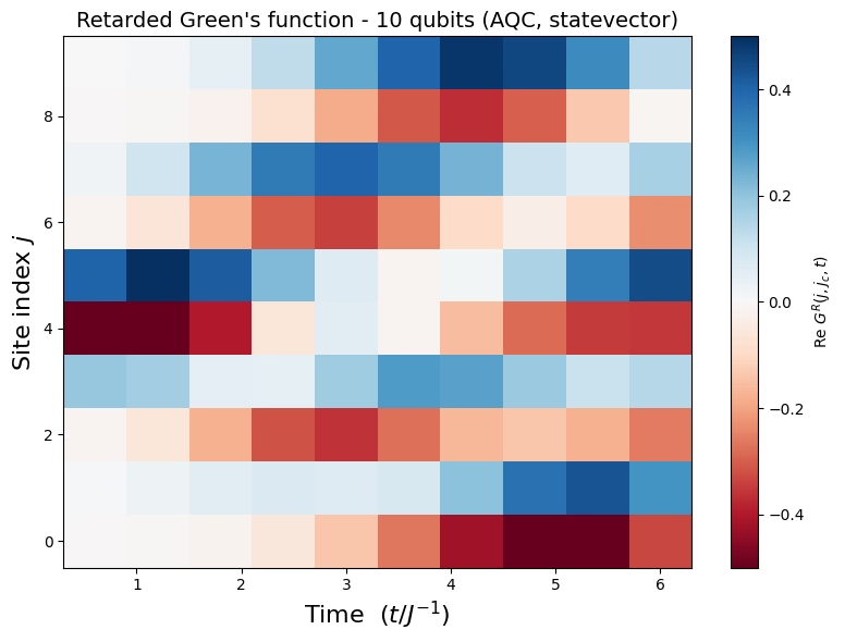
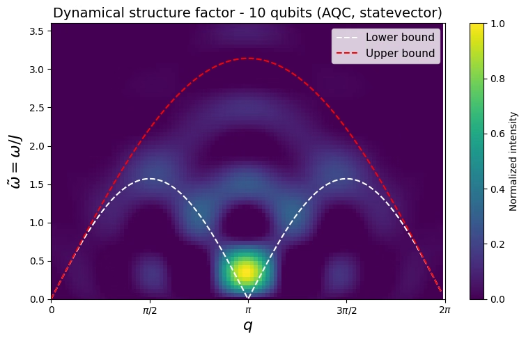
大規模ハードウェアの例

同じワークフローは、科学的なコードを何も変更することなくスケールアップします: 30サイトの鎖、2倍のTrotter深さ(20ステップ)、アンザッツの深さを変化させる圧縮計画(より後の、よりエンタングルした複雑なステップにはより深いアンザッツ)、そして関数に組み込まれた誤り軽減(ダイナミカル・デカップリング、パウリ・ツイリング、ツイリングされた読み出しエラー消去(TREX))を用いたIBM Quantumプロセッサ上での実行です。セットアップからのfnハンドルを再利用して、シミュレータの例と同じ4つのステップを順に見ていきます。

	小規模	大規模
量子ビット	10	30
Trotterステップ	10	20
AQC圧縮ステップ(1層 + 2層)	3 + 2 = 5	6 + 4 = 10
基底状態アンザッツ層	3	5
MPS最大ボンド次元	32	128
バックエンド	statevector	DD、パウリ・ツイリング、TREXを備えたQPU

ステップ1: 古典的な入力を量子問題にマッピングする

同じKCuF$_3$ハイゼンベルグSparsePauliOpを構築して基底状態を準備します。ここでは長い鎖に対応するため、より深いgs_layers=5アンザッツを使用し、その後、中心サイトに$\pi/2$ $Z$中性子キックを焼き込みます。これは小規模のマッピングと同一ですが、$n = 30$で行います。

10サイトの実行よりも低い基底状態忠実度が予想されます。ここではおよそ0.82に対し、より小さい鎖では0.98でした。これは5層のHVAでは30サイトの基底状態を完全に捉えられないためです。これは失敗ではなく想定内であり、元のチュートリアルでも同じ理由で50サイトの場合はおよそ0.65を許容しています。gs_layersやCOBYQAの反復回数上限を増やすと、追加の古典コストと引き換えに改善します。

n = 30
dt = 0.6
time_steps = 20
center = n // 2 - 1

# Same MPS settings as the original large-scale run: a larger bond for the
# longer, more-entangled chain (shared by GS prep and AQC compression).
mps_max_bond = 128
mps_cutoff = 1e-8

# Same KCuF3 Hamiltonian and ground-state prep, on a larger chain
H = SparsePauliOp.from_sparse_list(
    [(p, [i, i + 1], 0.25) for i in range(n - 1) for p in ("XX", "YY", "ZZ")],
    num_qubits=n,
)
gs_circuit = prepare_ground_state(
    n, gs_layers=5, max_bond=mps_max_bond, cutoff=mps_cutoff
)
gs_circuit.rz(np.pi / 2, center)  # neutron kick at the center site
print(
    f"Prepared {n}-qubit ground state with the neutron kick at site {center}."
)

DMRG ground-state energy: -13.111355
GS fidelity: 0.8201
Prepared 30-qubit ground state with the neutron kick at site 14.

ステップ2と3: 関数テンプレートを使って圧縮と実行を行う

シミュレータの例と同じ単一の呼び出しですが、今回はbackend_nameがIBM Quantumプロセッサを指しているため、関数はそこでトランスパイルと実行を行います。圧縮プランはアンザッツの深さを変えます。最初の6つの(低エンタングルメントの)トロッター・ステップは浅い単層アンザッツに圧縮され、次の4つはより深い2層アンザッツに圧縮され、20ステップのうち残りの10ステップは通常のトロッターとして実行されます。aqc_optionsは、より長くよりエンタングルした鎖に対応するため(元の設定に合わせて)、MPSボンド次元をmax_bond=128に引き上げ、同じL-BFGS-Bオプティマイザを100反復に制限したままにします。estimator_optionsは組み込みのエラー緩和を有効にします。動的デカップリング(XY4)、ゲート・トワイリング、TREX測定緩和です。関数のデフォルトは、TREX学習予算(measure_noise_learning)を除き、これらすべてにおいて既に元のチュートリアルと一致しています。呼び出し元が指定するestimator_optionsは関数のデフォルトにマージされるのではなく、丸ごと置き換えるため、キーを1つ省略するとIBM Quantum Computeのデフォルトに戻ってしまい、関数のデフォルトにはならないので、ブロック全体をここに書き出しています。

# Steps 2 + 3: the function compresses (varied ansatz) and executes on hardware.
job = fn.run(
    t_steps=time_steps,
    aqc_segments=[
        {
            "n_steps": 6,
            "ansatz_steps": 1,
        },  # early steps -> shallow 1-layer ansatz
        {
            "n_steps": 4,
            "ansatz_steps": 2,
        },  # later steps -> deeper 2-layer ansatz
    ],
    aqc_options={
        "max_bond": mps_max_bond,  # 128 for the longer chain
        "cutoff": mps_cutoff,
        "optimizer_settings": {
            "method": "L-BFGS-B",
            "jac": True,
            "options": {"maxiter": 100},
        },
    },
    dt=dt,
    hamiltonian=H,
    initial_state=gs_circuit,
    backend_name="ibm_pittsburgh",
    # Mitigation settings from the original tutorial. Only the two
    # measure_noise_learning values differ from the function's defaults; the rest
    # restates them, because a caller-supplied estimator_options dict replaces the
    # function's defaults wholesale rather than merging into them.
    estimator_options={
        "environment": {"job_tags": ["TUT-SNS"]},
        "dynamical_decoupling": {"enable": True, "sequence_type": "XY4"},
        "twirling": {
            "enable_gates": True,
            "num_randomizations": 1000,
            "shots_per_randomization": 128,
        },
        "resilience": {
            "measure_mitigation": True,
            "measure_noise_learning": {
                "num_randomizations": 32,
                "shots_per_randomization": 100,
            },
        },
    },
)
print("job ID (save this to reconnect later):", job.job_id)

job ID (save this to reconnect later): 43ed8d07-6d7d-4f33-b70a-7f31b765b310

長時間実行するジョブへの再接続

大規模な実行は迅速ではなく、時間の大半はQPU上ではなく古典計算に費やされます。AQC圧縮は何かがQPUに到達する前に関数内で実行されます。30サイトでmax_bond=128の場合、私たちの実行ではほぼ4時間かかりましたが、これはこのチュートリアル冒頭の使用量の見積もりに記載されているおよそ18分のQPU時間とは対照的です。キューの待機時間はこの両方に加算されます。実行中、このノートブックやカーネルを開いたままにしておく必要はありません。

直前のセルが出力したジョブIDをコピーして保存してください。次の3つのセルを使うと、後で処理を再開できます。

1. 再接続する。新しいカーネル・セッションでのみ必要です。セットアップのセルを再実行してserverlessを再作成し、保存したIDからjobハンドルを再構築してください。提出したセッションにまだいる場合、ハンドルは既に有効なため、このセルはスキップしてください。

2. ステータスを確認する。DONEと報告されるまで再実行してください。

3. 結果を取得する。ステータスがDONEになった時点で一度だけ実行してください。

次の再接続セルにはプレースホルダーが含まれています。ご自身のjob_idに置き換えてください。

# Reconnect to a previously submitted job by its ID. Only needed in a NEW kernel
# session; if you are still in the session where you submitted, the `job` handle
# from the preceding cell is already live, so skip this cell. Replace the ID that follows with your own.
job = serverless.get_job_by_id("<your job ID>")

# Check where the job is. Re-run this until it reports DONE before fetching the
# result in the following cell: QUEUED -> INITIALIZING -> RUNNING: OPTIMIZING_FOR_HARDWARE ->
# RUNNING: WAITING_FOR_QPU -> RUNNING: EXECUTING_QPU -> RUNNING: POST_PROCESSING
# -> DONE.
print(job.status())

DONE

# Run this only once the preceding status cell reports DONE. result() blocks until
# the job finishes, so calling it earlier just waits (possibly for hours).
result = job.result()
print(
    "AQC fidelities:",
    {k: round(v, 4) for k, v in result["metadata"]["aqc_fidelities"].items()},
)

ev = np.array(result["expectation_values"])
Gjjc = ev[1:]  # drop the t = 0 row -> shape (time_steps, n)

AQC fidelities: {'1': 1.0, '2': 0.9994, '3': 0.9944, '4': 0.9853, '5': 0.9747, '6': 0.959, '7': 0.9495, '8': 0.9542, '9': 0.9533, '10': 0.9451}

ステップ4: 望ましい古典形式で結果を後処理して返す

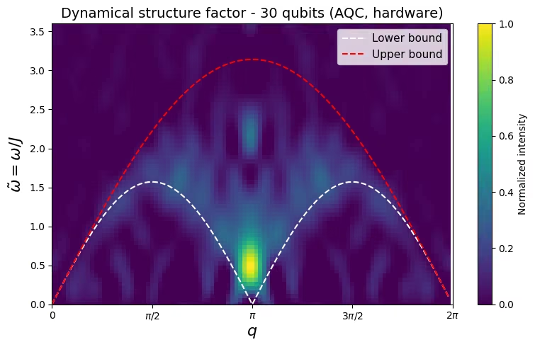
シミュレータ実行と同一の後処理です。グリーン関数をフーリエ変換して$S(q, \omega)$を得て、鏡映対称化し、負の値を切り取ります。より長い鎖と時間発展により、2スピノン連続体ははるかに良好に分解されます。破線の境界の間のバンドを埋め、$q = \pi$付近で最も明るくなるはずです。

n = result["metadata"]["n"]
q_res, w_res = 100, 100
spectrum = get_spectrum(n, Gjjc, dt, time_steps, q_res, w_res)
spectrum = -(spectrum + spectrum[:, ::-1]) / 2  # mirror symmetry
spectrum = np.clip(spectrum, a_min=0, a_max=None)  # clip negatives

plot_green(
    n,
    Gjjc,
    time_steps,
    dt,
    title=f"Retarded Green's function - {n} qubits (AQC, hardware)",
)
plot_spectrum(
    spectrum,
    dt,
    q_res,
    w_res,
    lower_bound=True,
    upper_bound=True,
    title=f"Dynamical structure factor - {n} qubits (AQC, hardware)",
)

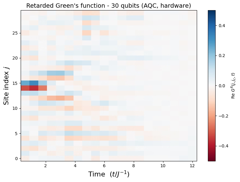
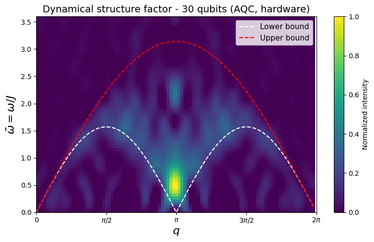
付録

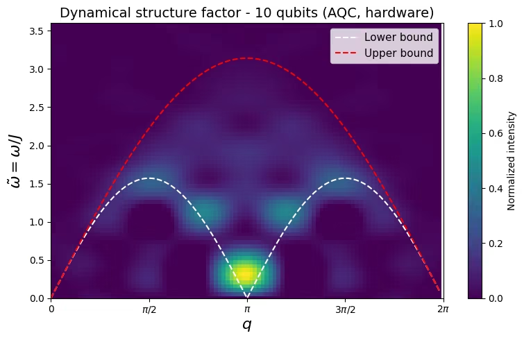
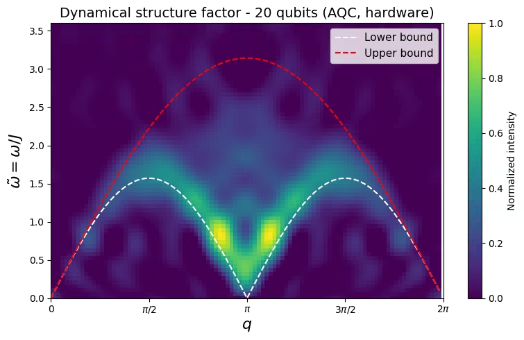
直前のハードウェアの例では単一の鎖長のみを実行しています。以降の3つのスペクトルは、ibm_pittsburgh上で10、20、30サイトについて、他のすべての入力を固定して(dt = 0.6の20トロッター・ステップ、6つの1層プラス4つの2層のAQC圧縮ステップという圧縮プラン、max_bond = 128)、この同じワークフローを以前に実行したハードウェアの結果から得られたものです。これらは記録された結果であり、直前のセルからの出力ではありません。

3つのサイズすべてで同じ設定が使われているため、スペクトルは直接比較可能です。例えば、鎖長ごとにより多くの基底状態アンザッツ層やより大きなmax_bondなどにチューニングすることで、ここで示した結果よりも良い結果が得られる可能性があります。

次のステップ

Recommendations

• このワークフローを自分自身のシステムに適用してください。この関数は任意の1次元最近接SparsePauliOpを受け付けるため、異なる鎖ハミルトニアン、初期状態、または観測量のセットでも同じPRE → FUNCTION → POSTパイプラインを実行できます。完全な入出力の契約については、GitHub上のAQC Dynamicsテンプレートを参照してください。

• このベンチマークの出典となる論文を読んでください。Lee他、中性子散乱実験による量子シミュレーションのベンチマーク (arXiv:2603.15608)。

• 元の「中性子散乱をシミュレートする」チュートリアルと比較してください。これは、このチュートリアルがデプロイされた関数テンプレートに移植したインライン・ワークフローです。

• ハードウェア実行に適用されたエラー緩和・抑制手法についてさらに深く学んでください。動的デカップリング、パウリ・トワイリング、TREXです。