サンプルベース量子対角化による化学ハミルトニアンの解析
使用量の目安: Heron r2 プロセッサで1分未満(注: これはあくまで目安です。実際の実行時間は異なる場合があります。)
学習成果
このチュートリアルを通じて、ユーザーは以下を理解できるようになります:
- 量子処理ユニット(QPU)からサンプリングしたビット列を使用して、SQD Qiskit アドオンで分子系の基底状態エネルギーを近似する方法。
- ffsimを使用して量子化学シミュレーション用の局所ユニタリクラスターヤストロー(LUCJ)回路を構築する方法。
前提条件
このチュートリアルを始める前に、以下のトピックについて理解しておくことを推奨します:
- 量子化学と第二量子化
- 量子回路からサンプリングするためのSampler プリミティブの使用方法
背景
このチュートリアルでは、SQD Qiskit アドオンを使用してサンプルベース量子対角化(SQD)アルゴリズムを実装し、ノイズのある量子サンプルを後処理することで平衡結合長における窒素分子 の基底状態の近似を求める方法を示します。ソフトウェアの詳細は対応するドキュメントに記載されており、簡単な例から始めることもできます。
このチュートリアルは、量子化学(特に分子の基底状態エネルギーの探索)に精通したユーザーを対象としています。ワークフローの詳細なウォークスルーについては、量子対角化アルゴリズムコースを参照してください。
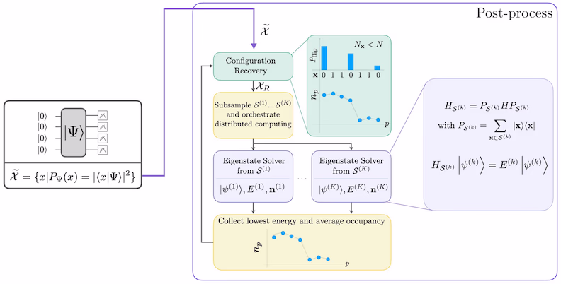
SQDは、量子システムのハミルトニアンなどの量子演算子の固有値と固有ベクトルを、量子コンピューティングと分散古典コンピューティングを組み合わせて求める手法です。古典分散コンピューティングは、量子プロセッサから得られたサンプルを処理し、それらが張る部分空間にターゲットハミルトニアンを射影して対角化するために使用されます。SQDベースのワークフローは以下のステップで構成されます:
- 回路アンザッツを選択し、参照状態(この場合は Hartree-Fock 状態)に対して量子コンピュータ上で適用します。
- 得られた量子状態からビット列をサンプリングします。
- ビット列に対して自己無撞着配置回復手順を実行し、基底状態の近似を取得します。
SQDは、ターゲット固有状態がスパースである場合にうまく機能することが知られています。つまり、波動関数が計算基底状態の集合 で支持されており、そのサイズが問題のサイズに対して指数的に増大しない場合です。
量子化学
分子系のハミルトニアンは次のように記述できます。
ここで、 と は分子積分と呼ばれる複素数であり、コンピュータプログラムを使用して分子の仕様から計算することができます。このチュートリアルでは、PySCF ソフトウェアパッケージを使用して積分を計算します。
分子ハミルトニアンの導出の詳細については、量子化学の教科書(例えば、Szabo と Ostlund 著 Modern Quantum Chemistry)を参照してください。量子化学問題が量子コンピュータにどのようにマッピングされるかの概要については、Qiskit Global Summer School 2024 の講義 Mapping Problems to Qubits を参照してください。
局所ユニタリクラスターヤストロー(LUCJ)アンザッツ
SQDではサンプルを抽出するための量子回路アンザッツが必要です。このチュートリアルでは、物理的な動機付けとハードウェア親和性の両方を兼ね備えた局所ユニタリクラスターヤストロー(LUCJ)アンザッツを使用します。アンザッツ回路の構築には ffsim を使用します。
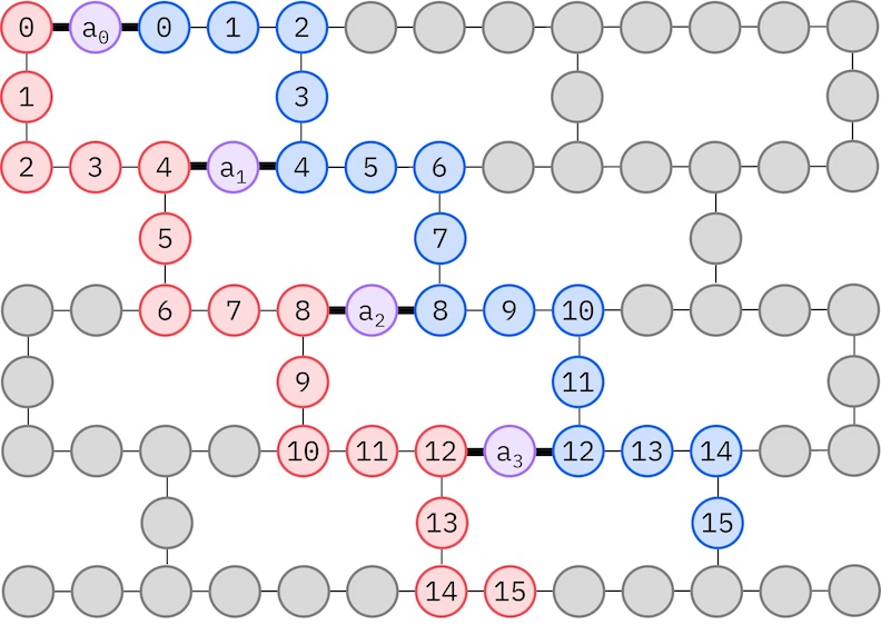
LUCJアンザッツは、制限されたQubit接続性を持つQPUに適応します。スピン軌道は、アンザッツがSWAPゲートによるルーティングを必要としないようにQubitsにマッピングされます。IBM® ハードウェアはヘビーヘックス格子量子ビットトポロジーを持っており、この場合は以下に示す「ジグザグ」パターンを採用できます。このパターンでは、同じスピンを持つ軌道は線形トポロジーの量子ビットにマッピングされ(赤と青の円)、異なるスピンの軌道間の接続は4番目の空間軌道ごとに存在し、補助量子ビット(紫の円)を介して接続が行われます。
自己無撞着配置回復
自己無撞着配置回復手順は、ノイズのある量子サンプルからできる限り多くの信号を抽出するために設計されています。分子ハミルトニアンは粒子数とスピンZを保存するため、これらの対称性も保存する回路アンザッツを選択することが合理的です。Hartree-Fock状態に適用した場合、ノイズがない設定では、得られる状態は固定された粒子数とスピンZを持ちます。したがって、この状態からサンプリングされた任意のビット列のスピン- 半分とスピン- 半分は、Hartree-Fock状態と同じハミング重みを持つはずです。現在の量子プロセッサにはノイズが存在するため、測定されたビット列の一部はこの性質に違反します。単純なポストセレクションではこれらのビット列を破棄しますが、それらのビット列にはまだ何らかの信号が含まれている可能性があるため、これは無駄です。自己無撞着回復手順は、後処理でその信号の一部を回復しようとするものです。この手順は反復的であり、入力として基底状態における各軌道の平均占有数の推定値が必要で、まず生のサンプルから計算されます。手順はループ内で実行され、各反復は以下のステップで構成されます:
- 指定された対称性に違反する各ビット列について、現在の平均軌道占有数の推定値にビット列を近づけるように設計された確率的手順でビットを反転させ、新しいビット列を取得します。
- 対称性を満たすすべての古いビット列と新しいビット列を収集し、事前に選択した固定サイズの部分集合をサブサンプリングします。
- 各ビット列の部分集合について、対応する基底ベクトルが張る部分空間にハミルトニアンを射影し(これらの基底ベクトルの説明は前のセクションを参照)、古典コンピュータ上で射影ハミルトニアンの基底状態推定を計算します。
- 最もエネルギーが低い基底状態推定で、平均軌道占有数の推定値を更新します。
SQDワークフロー図
SQDワークフローは以下の図に示されています:
要件
このチュートリアルを開始する前に、以下がインストールされていることを確認してください:
- Qiskit SDK v1.0 以降、visualization サポート付き
- Qiskit Runtime v0.22 以降(
pip install qiskit-ibm-runtime) - SQD Qiskit アドオン v0.11 以降(
pip install qiskit-addon-sqd) - ffsim v0.0.75 以降(
pip install ffsim)
セットアップ
# Added by doQumentation — required packages for this notebook
!pip install -q ffsim matplotlib numpy pyscf qiskit qiskit-addon-sqd qiskit-ibm-runtime
import math

import ffsim
import matplotlib.pyplot as plt
import numpy as np
import pyscf
import pyscf.cc
import pyscf.mcscf
from qiskit import QuantumCircuit, QuantumRegister
from qiskit.primitives import StatevectorSampler
from qiskit.providers.fake_provider import GenericBackendV2
from qiskit_ibm_runtime import QiskitRuntimeService
from qiskit_ibm_runtime import SamplerV2 as Sampler
小規模シミュレーターの例
このチュートリアルでは、平衡結合距離付近の窒素分子の基底状態の近似を求めます。まず、実験をシミュレートして動作確認ができるよう、小規模なSTO-6G基底セットを使用します。
ステップ 1: 古典的な入力を量子問題にマッピングする
まず、分子とその性質を指定します。
# Specify molecule properties
spin_sq = 0

# Build N2 molecule
mol = pyscf.gto.Mole()
mol.build(
    atom=[["N", (0, 0, 0)], ["N", (1.0, 0, 0)]],
    basis="sto-6g",
    symmetry="Dooh",
)

# Define active space
n_frozen = 2
active_space = range(n_frozen, mol.nao_nr())

# Get molecular integrals
scf = pyscf.scf.RHF(mol).run()
norb = len(active_space)
n_electrons = int(sum(scf.mo_occ[active_space]))
n_alpha = (n_electrons + mol.spin) // 2
n_beta = (n_electrons - mol.spin) // 2
nelec = (n_alpha, n_beta)
cas = pyscf.mcscf.CASCI(scf, norb, nelec)
mo = cas.sort_mo(active_space, base=0)
hcore, nuclear_repulsion_energy = cas.get_h1cas(mo)
eri = pyscf.ao2mo.restore(1, cas.get_h2cas(mo), norb)

# Compute exact energy using FCI
reference_energy = cas.run().e_tot

print(f"norb = {norb}")
print(f"nelec = {nelec}")
converged SCF energy = -108.464957764796
CASCI E = -108.595987350986  E(CI) = -32.4115475088426  S^2 = 0.0000000
norb = 8
nelec = (5, 5)
LUCJアンザッツ回路を構築する前に、まず以下のコードセルでCCSD計算を実行します。この計算から得られる および 振幅 は、アンザッツのパラメータの初期化に使用されます。
# Get CCSD t2 amplitudes for initializing the ansatz
ccsd = pyscf.cc.CCSD(
    scf, frozen=[i for i in range(mol.nao_nr()) if i not in active_space]
).run()
t1 = ccsd.t1
t2 = ccsd.t2
E(CCSD) = -108.5933309085008 E_corr = -0.1283731437052354
次に、ffsim を使用してアンザッツ回路を作成します。この分子は閉殻Hartree-Fock状態を持つため、UCJアンザッツのスピンバランス型変種である UCJOpSpinBalanced を使用します。from_t_amplitudes メソッドで optimize=True を設定して、 振幅の「圧縮」二重因子分解を有効にします(詳細はffismのドキュメントの The local unitary cluster Jastrow (LUCJ) ansatz を参照してください)。
LUCJアンザッツはQPUの利用可能な接続性に適応するため、アンザッツを作成する前にQPUバックエンドを初期化する必要があります。ここでは、ヘビーヘックスカップリングマップとLUCJアンザッツが自然に分解されるゲートセットを持つ汎用バックエンドを作成します。次に、ffsim.qiskit.generate_lucj_pass_manager を使用して、LUCJアンザッツに関する背景セクションで説明した「ジグザグ」レイアウトに従って、LUCJアンザッツを指定バックエンドにトランスパイルするための特化パスマネージャを作成します。この関数は、選択したレイアウトに関連するエラーを最小化するスコアリングヒューリスティックを使用しており、バックエンドが実際のQPUやノイズモデルを持つシミュレーターの場合に重要です。パスマネージャを返すほか、ハードウェア上で実装できるアルファ・ベータカップリングペアも返します。すべてのペアを実装できない場合は警告が出力されます。
import warnings

from qiskit.transpiler import CouplingMap

warnings.formatwarning = lambda msg, *args, **kwargs: f"Warning: {msg}\n"

# Set ansatz properties
n_reps = 1
pairs_aa = [(p, p + 1) for p in range(norb - 1)]

# Let generate_lucj_pass_manager determine the alpha-beta interactions
pairs_ab = None

# Initialize backend
coupling_map = CouplingMap.from_heavy_hex(3)
backend = GenericBackendV2(
    coupling_map.size(),
    coupling_map=coupling_map,
    basis_gates=["cp", "xx_plus_yy", "p", "x", "swap"],
)

# Create pass manager
pass_manager, pairs_ab = ffsim.qiskit.generate_lucj_pass_manager(
    backend=backend,
    norb=norb,
    connectivity="heavy-hex",
    interaction_pairs=(pairs_aa, pairs_ab),
    optimization_level=3,
)

# Create the LUCJ ansatz operator
ucj_op = ffsim.UCJOpSpinBalanced.from_t_amplitudes(
    t2=t2,
    t1=t1,
    n_reps=n_reps,
    interaction_pairs=(pairs_aa, pairs_ab),
    # Setting optimize=True enables the "compressed" factorization
    optimize=True,
    # Limit the number of optimization iterations to prevent the code cell
    # from running too long. Removing this line may improve results.
    options=dict(maxiter=1000),
)

# create an empty quantum circuit
qubits = QuantumRegister(2 * norb, name="q")
circuit = QuantumCircuit(qubits)

# prepare Hartree-Fock state as the reference state and append it
# to the quantum circuit
circuit.append(ffsim.qiskit.PrepareHartreeFockJW(norb, nelec), qubits)

# apply the UCJ operator to the reference state
circuit.append(ffsim.qiskit.UCJOpSpinBalancedJW(ucj_op), qubits)
circuit.measure_all()
ステップ 2: 量子ハードウェア実行のために最適化する
次に、ターゲットハードウェアに対して回路を最適化します。通常、このステップではハードウェアバックエンドとそのバックエンド用のパスマネージャを初期化しますが、LUCJアンザッツはハードウェアの接続性に適応しているため、これらの処理はすでに前のステップで行いました。残るのは、パスマネージャを回路に対して実行して、QPU上で直接実行できるISA回路にトランスパイルすることだけです。
isa_circuit = pass_manager.run(circuit)
print(f"Gate counts: {isa_circuit.count_ops()}")
Gate counts: OrderedDict({'xx_plus_yy': 86, 'p': 16, 'measure': 16, 'cp': 15, 'x': 10, 'swap': 2, 'barrier': 1})
ステップ 3: Qiskit プリミティブを使用して実行する
ハードウェア実行用に回路を最適化した後、ターゲットハードウェア上で回路を実行し、基底状態エネルギー推定のためのサンプルを収集する準備が整います。回路は1つだけなので、Qiskit Runtime の ジョブ実行モード を使用して回路を実行します。
rng = np.random.default_rng()
sampler = StatevectorSampler(seed=rng)
job = sampler.run([isa_circuit], shots=100_000)
Warning: Trying to add QuantumRegister to a QuantumCircuit having a layout
primitive_result = job.result()
pub_result = primitive_result[0]
ステップ 4: 後処理を行い、結果を所望の古典フォーマットで返す
QPU出力の品質を判断する有用な指標は、返された有効な配置の数です。有効な配置とは、正しい粒子数とスピンZを持つもので、ビット列の右半分のハミング重みがスピンアップ電子数に等しく、左半分のハミング重みがスピンダウン電子数に等しいことを意味します。次のセルでは、サンプリングされた配置のうち有効なものの割合を計算します。
def is_valid_bitstring(
    bitstring: str, norb: int, nelec: tuple[int, int]
) -> bool:
    n_alpha, n_beta = nelec
    return (
        len(bitstring) == 2 * norb
        and bitstring[norb:].count("1") == n_alpha
        and bitstring[:norb].count("1") == n_beta
    )

bit_array = pub_result.data.meas
num_valid = sum(
    is_valid_bitstring(b, norb, nelec) for b in bit_array.get_bitstrings()
)
valid_fraction = num_valid / bit_array.num_shots
print(f"Fraction of sampled configurations that are valid: {valid_fraction}")
Fraction of sampled configurations that are valid: 1.0
すべてのビット列が有効なのは、ノイズのないシミュレーター上で回路をサンプリングしているためです。ノイズのあるQPU上で実行する場合、この割合は1未満になりますが、以下のセルで計算されるようにビット列が一様ランダムにサンプリングされた場合に期待される割合よりも大きくなることが望まれます。
expected_fraction_random = (
    math.comb(norb, n_alpha) * math.comb(norb, n_beta) / 2 ** (2 * norb)
)
print(
    f"Expected fraction of valid configurations from uniformly random bitstrings: "
    f"{expected_fraction_random}"
)
Expected fraction of valid configurations from uniformly random bitstrings: 0.0478515625
次に、diagonalize_fermionic_hamiltonian 関数を使用してハミルトニアンの基底状態エネルギーを推定します。この関数は、自己無撞着配置回復(self-consistent configuration recovery)手続きを実行し、ノイズを含む量子サンプルを反復的に改善してエネルギー推定値の精度を向上させます。中間結果を後の解析のために保存できるよう、コールバック関数を渡します。diagonalize_fermionic_hamiltonian の引数の説明については、API ドキュメント を参照してください。
ここでは、diagonalize_fermionic_hamiltonian の initial_occupancies 引数を使用して、基底状態における軌道占有数の初期推定値としてHartree-Fock配置を指定します。このアプローチは、基底状態がHartree-Fock配置に有意なサポートを持つ系には適切ですが、他の状況では適切でない場合もあります。そのような場合は、より高度な計算手法によってより良い初期推定値が得られる場合があります。initial_occupancies を指定することで、有効な配置がサンプリングされなかった場合でも配置回復を実行できます(大規模な回路をノイズのあるQPUでサンプリングする際にこのようなことが起こり得ます)。この引数がない場合、有効な配置が提供されなければ配置回復は失敗してエラーを発生させます。
from functools import partial

from qiskit_addon_sqd.fermion import (
    SCIResult,
    diagonalize_fermionic_hamiltonian,
    solve_sci_batch,
)

# SQD options
energy_tol = 1e-3
occupancies_tol = 1e-3
max_iterations = 5

# Eigenstate solver options
num_batches = 3
samples_per_batch = 300
symmetrize_spin = True
carryover_threshold = 1e-4
max_cycle = 200

# Use the Hartree-Fock configuration as an initial guess for the orbital occupancies
initial_occupancies = (
    np.array([1] * n_alpha + [0] * (norb - n_alpha)),
    np.array([1] * n_beta + [0] * (norb - n_beta)),
)

# Pass options to the built-in eigensolver. If you just want to use the defaults,
# you can omit this step, in which case you would not specify the sci_solver argument
# in the call to diagonalize_fermionic_hamiltonian below.
sci_solver = partial(solve_sci_batch, spin_sq=0.0, max_cycle=max_cycle)

# List to capture intermediate results
result_history = []

def callback(results: list[SCIResult]):
    result_history.append(results)
    iteration = len(result_history)
    print(f"Iteration {iteration}")
    for i, result in enumerate(results):
        print(f"\tSubsample {i}")
        print(f"\t\tEnergy: {result.energy + nuclear_repulsion_energy}")
        print(
            f"\t\tSubspace dimension: {np.prod(result.sci_state.amplitudes.shape)}"
        )

result = diagonalize_fermionic_hamiltonian(
    hcore,
    eri,
    bit_array,
    samples_per_batch=samples_per_batch,
    norb=norb,
    nelec=nelec,
    num_batches=num_batches,
    energy_tol=energy_tol,
    occupancies_tol=occupancies_tol,
    max_iterations=max_iterations,
    sci_solver=sci_solver,
    symmetrize_spin=symmetrize_spin,
    initial_occupancies=initial_occupancies,
    carryover_threshold=carryover_threshold,
    callback=callback,
    seed=rng,
)

final_energy = result.energy + nuclear_repulsion_energy
energy_error = final_energy - reference_energy
print(f"Final energy: {final_energy}")
print(f"Final energy error: {energy_error}")
Iteration 1
	Subsample 0
		Energy: -108.59275573641656
		Subspace dimension: 900
	Subsample 1
		Energy: -108.59275573641656
		Subspace dimension: 900
	Subsample 2
		Energy: -108.59275573641656
		Subspace dimension: 900
Iteration 2
	Subsample 0
		Energy: -108.59275573641656
		Subspace dimension: 900
	Subsample 1
		Energy: -108.59275573641656
		Subspace dimension: 900
	Subsample 2
		Energy: -108.59275573641656
		Subspace dimension: 900
Final energy: -108.59275573641656
Final energy error: 0.0032316145694579745
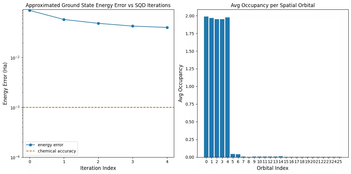
結果の可視化
最初のプロットは、このシミュレーションでは最初の反復後に既に 1 mH 以内の精度に達していることを示しています(化学精度は一般に 1 kcal/mol 1.6 mH とされています)。ただし、これは小規模な系であり、サンプルがノイズレスであるため配置回復は必要ありません。より大規模な系をノイズのあるQPU上で実行した場合は、複数回の配置回復反復が必要になることがあり、最終的な精度が悪化する場合があります。一般的に、配置回復の反復回数を増やすか、バッチあたりのサンプル数を増やすことで、エネルギーの精度をさらに向上させることができます。
2番目のプロットは、最終反復後の各空間軌道の平均占有数を示しています。スピンアップ電子とスピンダウン電子の両方が、解において高い確率で最初の5つの軌道を占有していることがわかります。
# Data for energies plot
x1 = range(len(result_history))
min_e = [
    min(result, key=lambda res: res.energy).energy + nuclear_repulsion_energy
    for result in result_history
]
e_diff = [abs(e - reference_energy) for e in min_e]
yt1 = [1.0, 1e-1, 1e-2, 1e-3, 1e-4]

# Chemical accuracy (+/- 1 milli-Hartree)
chem_accuracy = 0.001

# Data for avg spatial orbital occupancy
y2 = np.sum(result.orbital_occupancies, axis=0)
x2 = range(len(y2))

fig, axs = plt.subplots(1, 2, figsize=(12, 6))

# Plot energies
axs[0].plot(x1, e_diff, label="energy error", marker="o")
axs[0].set_xticks(x1)
axs[0].set_xticklabels(x1)
axs[0].set_yticks(yt1)
axs[0].set_yticklabels(yt1)
axs[0].set_yscale("log")
axs[0].set_ylim(1e-4)
axs[0].axhline(
    y=chem_accuracy,
    color="#BF5700",
    linestyle="--",
    label="chemical accuracy",
)
axs[0].set_title("Approximated Ground State Energy Error vs SQD Iterations")
axs[0].set_xlabel("Iteration Index", fontdict={"fontsize": 12})
axs[0].set_ylabel("Energy Error (Ha)", fontdict={"fontsize": 12})
axs[0].legend()

# Plot orbital occupancy
axs[1].bar(x2, y2, width=0.8)
axs[1].set_xticks(x2)
axs[1].set_xticklabels(x2)
axs[1].set_title("Avg Occupancy per Spatial Orbital")
axs[1].set_xlabel("Orbital Index", fontdict={"fontsize": 12})
axs[1].set_ylabel("Avg Occupancy", fontdict={"fontsize": 12})

plt.tight_layout()
plt.show()

大規模ハードウェアの例
次に、実際の量子ハードウェア上でより大規模な例を実行します。ここでは、cc-pVDZ基底セットから窒素分子の活性空間を導出します。
ステップ 1〜4
ここでは、すべてのステップを1つのワークフローにまとめてより大規模なスケールで実行します。これを実際の量子ハードウェア上で実行します。
# ------------------------------ Step 1 ------------------------------
# Build N2 molecule
mol = pyscf.gto.Mole()
mol.build(
    atom=[["N", (0, 0, 0)], ["N", (1.0, 0, 0)]],
    basis="cc-pvdz",
    symmetry="Dooh",
)

# Define active space
n_frozen = 2
active_space = range(n_frozen, mol.nao_nr())

# Get molecular integrals
scf = pyscf.scf.RHF(mol).run()
norb = len(active_space)
n_electrons = int(sum(scf.mo_occ[active_space]))
n_alpha = (n_electrons + mol.spin) // 2
n_beta = (n_electrons - mol.spin) // 2
nelec = (n_alpha, n_beta)
cas = pyscf.mcscf.CASCI(scf, norb, nelec)
mo = cas.sort_mo(active_space, base=0)
hcore, nuclear_repulsion_energy = cas.get_h1cas(mo)
eri = pyscf.ao2mo.restore(1, cas.get_h2cas(mo), norb)

# Store reference energy from SCI calculation performed separately
reference_energy = -109.22802921665716

print(f"norb = {norb}")
print(f"nelec = {nelec}")

# Get CCSD t2 amplitudes for initializing the ansatz
ccsd = pyscf.cc.CCSD(
    scf, frozen=[i for i in range(mol.nao_nr()) if i not in active_space]
).run()
t1 = ccsd.t1
t2 = ccsd.t2

# Set ansatz properties
n_reps = 1
pairs_aa = [(p, p + 1) for p in range(norb - 1)]

# Let generate_lucj_pass_manager determine the alpha-beta interactions
pairs_ab = None

# Initialize backend
service = QiskitRuntimeService()
backend = service.least_busy(
    operational=True, simulator=False, min_num_qubits=133
)
print(f"Using backend {backend.name}")

# Create pass manager
pass_manager, pairs_ab = ffsim.qiskit.generate_lucj_pass_manager(
    backend=backend,
    norb=norb,
    connectivity="heavy-hex",
    interaction_pairs=(pairs_aa, pairs_ab),
    optimization_level=3,
)

# Create the LUCJ ansatz operator
ucj_op = ffsim.UCJOpSpinBalanced.from_t_amplitudes(
    t2=t2,
    t1=t1,
    n_reps=n_reps,
    interaction_pairs=(pairs_aa, pairs_ab),
    # Setting optimize=True enables the "compressed" factorization
    optimize=True,
    # Limit the number of optimization iterations to prevent the code cell
    # from running too long. Removing this line may improve results.
    options=dict(maxiter=1000),
)

# create an empty quantum circuit
qubits = QuantumRegister(2 * norb, name="q")
circuit = QuantumCircuit(qubits)

# prepare Hartree-Fock state as the reference state and append it
# to the quantum circuit
circuit.append(ffsim.qiskit.PrepareHartreeFockJW(norb, nelec), qubits)

# apply the UCJ operator to the reference state
circuit.append(ffsim.qiskit.UCJOpSpinBalancedJW(ucj_op), qubits)
circuit.measure_all()

# ------------------------------ Step 2 ------------------------------

isa_circuit = pass_manager.run(circuit)
print(f"Gate counts: {isa_circuit.count_ops()}")

# ------------------------------ Step 3 ------------------------------
sampler = Sampler(mode=backend)
sampler.options.environment.job_tags = ["TUT_SQD"]
job = sampler.run([isa_circuit], shots=100_000)
primitive_result = job.result()
pub_result = primitive_result[0]

# ------------------------------ Step 4 ------------------------------

bit_array = pub_result.data.meas
num_valid = sum(
    is_valid_bitstring(b, norb, nelec) for b in bit_array.get_bitstrings()
)
valid_fraction = num_valid / bit_array.num_shots
print(f"Fraction of sampled configurations that are valid: {valid_fraction}")
expected_fraction_random = (
    math.comb(norb, n_alpha) * math.comb(norb, n_beta) / 2 ** (2 * norb)
)
print(
    f"Expected fraction of valid configurations from uniformly random bitstrings: "
    f"{expected_fraction_random}"
)
# SQD options
energy_tol = 1e-3
occupancies_tol = 1e-3
max_iterations = 5

# Eigenstate solver options
num_batches = 3
samples_per_batch = 300
symmetrize_spin = True
carryover_threshold = 1e-4
max_cycle = 200

# Use the Hartree-Fock configuration as an initial guess for the
# orbital occupancies
initial_occupancies = (
    np.array([1] * n_alpha + [0] * (norb - n_alpha)),
    np.array([1] * n_beta + [0] * (norb - n_beta)),
)

# Pass options to the built-in eigensolver. If you just want to use the defaults,
# you can omit this step, in which case you would not specify the
# sci_solver argument in the call to diagonalize_fermionic_hamiltonian below.
sci_solver = partial(solve_sci_batch, spin_sq=0.0, max_cycle=max_cycle)

# List to capture intermediate results
result_history = []

result = diagonalize_fermionic_hamiltonian(
    hcore,
    eri,
    bit_array,
    samples_per_batch=samples_per_batch,
    norb=norb,
    nelec=nelec,
    num_batches=num_batches,
    energy_tol=energy_tol,
    occupancies_tol=occupancies_tol,
    max_iterations=max_iterations,
    sci_solver=sci_solver,
    symmetrize_spin=symmetrize_spin,
    initial_occupancies=initial_occupancies,
    carryover_threshold=carryover_threshold,
    callback=callback,
    seed=rng,
)

final_energy = result.energy + nuclear_repulsion_energy
energy_error = final_energy - reference_energy
print(f"Final energy: {final_energy}")
print(f"Final energy error: {energy_error}")

# Data for energies plot
x1 = range(len(result_history))
min_e = [
    min(result, key=lambda res: res.energy).energy + nuclear_repulsion_energy
    for result in result_history
]
e_diff = [abs(e - reference_energy) for e in min_e]
yt1 = [1.0, 1e-1, 1e-2, 1e-3, 1e-4]

# Chemical accuracy (+/- 1 milli-Hartree)
chem_accuracy = 0.001

# Data for avg spatial orbital occupancy
y2 = np.sum(result.orbital_occupancies, axis=0)
x2 = range(len(y2))

fig, axs = plt.subplots(1, 2, figsize=(12, 6))

# Plot energies
axs[0].plot(x1, e_diff, label="energy error", marker="o")
axs[0].set_xticks(x1)
axs[0].set_xticklabels(x1)
axs[0].set_yticks(yt1)
axs[0].set_yticklabels(yt1)
axs[0].set_yscale("log")
axs[0].set_ylim(1e-4)
axs[0].axhline(
    y=chem_accuracy,
    color="#BF5700",
    linestyle="--",
    label="chemical accuracy",
)
axs[0].set_title("Approximated Ground State Energy Error vs SQD Iterations")
axs[0].set_xlabel("Iteration Index", fontdict={"fontsize": 12})
axs[0].set_ylabel("Energy Error (Ha)", fontdict={"fontsize": 12})
axs[0].legend()

# Plot orbital occupancy
axs[1].bar(x2, y2, width=0.8)
axs[1].set_xticks(x2)
axs[1].set_xticklabels(x2)
axs[1].set_title("Avg Occupancy per Spatial Orbital")
axs[1].set_xlabel("Orbital Index", fontdict={"fontsize": 12})
axs[1].set_ylabel("Avg Occupancy", fontdict={"fontsize": 12})

plt.tight_layout()
plt.show()
converged SCF energy = -108.929838385609
norb = 26
nelec = (5, 5)
E(CCSD) = -109.2177884185544  E_corr = -0.2879500329450045
Using backend ibm_boston
Warning: Backend cannot accommodate pairs_ab=[(0, 0), (4, 4), (8, 8), (12, 12), (16, 16), (20, 20), (24, 24)].
Removing interaction (24, 24) from the end.
Warning: Backend cannot accommodate pairs_ab=[(0, 0), (4, 4), (8, 8), (12, 12), (16, 16), (20, 20)].
Removing interaction (20, 20) from the end.
Gate counts: OrderedDict({'sx': 7039, 'rz': 6990, 'cz': 1858, 'x': 61, 'measure': 52, 'barrier': 1})
Fraction of sampled configurations that are valid: 0.02124
Expected fraction of valid configurations from uniformly random bitstrings: 9.607888706852918e-07
Iteration 1
	Subsample 0
		Energy: -109.13889134249762
		Subspace dimension: 120409
	Subsample 1
		Energy: -109.11785470455858
		Subspace dimension: 110889
	Subsample 2
		Energy: -109.13234360554011
		Subspace dimension: 130321
Iteration 2
	Subsample 0
		Energy: -109.16392179579177
		Subspace dimension: 223729
	Subsample 1
		Energy: -109.16281938332986
		Subspace dimension: 223729
	Subsample 2
		Energy: -109.16955816711932
		Subspace dimension: 233289
Iteration 3
	Subsample 0
		Energy: -109.17905772999075
		Subspace dimension: 324900
	Subsample 1
		Energy: -109.17532445048462
		Subspace dimension: 357604
	Subsample 2
		Energy: -109.1733168689756
		Subspace dimension: 348100
Iteration 4
	Subsample 0
		Energy: -109.18437778820451
		Subspace dimension: 474721
	Subsample 1
		Energy: -109.18450164209159
		Subspace dimension: 476100
	Subsample 2
		Energy: -109.18493571190754
		Subspace dimension: 487204
Iteration 5
	Subsample 0
		Energy: -109.18616522497996
		Subspace dimension: 622521
	Subsample 1
		Energy: -109.18652868888333
		Subspace dimension: 644809
	Subsample 2
		Energy: -109.18753326484406
		Subspace dimension: 585225
Final energy: -109.18753326484406
Final energy error: 0.040495951813099396
次のステップ
この研究が興味深いと感じた方は、以下の資料も参照してください:
- フェルミオン格子モデルのサンプルベース量子Krylov対角化 - 変分アンザッツの代わりに時間発展回路を使用した関連チュートリアル
- Diceソルバーを使用したSQD化学ワークフローのスケールアップ - より効率的なDiceソフトウェアを対角化に使用する方法を示すページ
- SQDアドオンAPIドキュメント -
diagonalize_fermionic_hamiltonian関数のリファレンス - Chemistry beyond the scale of exact diagonalization on a quantum-centric supercomputer - このチュートリアルの基となった論文