ノイズのある量子プロセッサ上での頑健かつコヒーレントな非可換ハドロン・ダイナミクスの観測
使用量の目安:Heron プロセッサ(ibm_boston またはそれと同等のもの)で約6分(注:これはあくまで目安です。実際の実行時間は異なる場合があります。)
学習の成果
-
非可換格子ゲージ理論(具体的には SU(2))を、効率的な量子シミュレーションのために Loop-String-Hadron(LSH)フレームワークを用いてどのように再定式化できるか
-
近似的な SU(2) ゲージ理論ハミルトニアンに対するトロッター化された時間発展回路を構築し、それを量子ビットにマッピングする方法
-
読み出しエラー抑制を伴う Qiskit Estimator プリミティブを使用して、これらの回路を IBM Quantum® ハードウェア上で実行する方法
前提条件
-
量子場理論の概念に関する基本的な理解(あれば役立ちますが必須ではありません。背景セクションで要点を説明します)
背景
動機
量子色力学(QCD)は、強い力の SU(3) ゲージ理論であり、クォークをハドロンに束縛し、閉じ込めと弦の切断を支配します。古典的な格子 QCD 手法は静的な性質の計算には優れていますが、符号問題のためにリアルタイムのダイナミクスをシミュレートすることはできません。量子コンピュータは、ゲージ場の自由度を量子ビットに直接エンコードすることで、この障壁を回避する手段を提供します。
このチュートリアルでは、そのようなシミュレーションを実演します。IBM Quantum ハードウェアを使用して、(1+1) 次元 SU(2) 格子ゲージ理論 — 最も単純な非可換ゲージ理論であり、完全な QCD への足がかりとなるもの — におけるリアルタイムのハドロン伝播をシミュレートします。
コグート・サスキンド・ハミルトニアン
この理論は、サイト上にスタッガード・フェルミオン(物質)を、リンク上に SU(2) ゲージ場を配置した1次元空間格子上で定式化されます。無次元形式に再スケーリングした後、ハミルトニアンは次の通りです:
ここで、 は色電場エネルギー、 はスタッガード質量項、 は物質・ゲージ相互作用(ホッピング)項であり、 はフェルミオン質量を表し、 は相互作用強度です。この理論の連続極限は かつ にあります。
Loop-String-Hadron(LSH)フレームワーク
主要な課題は、各リンク上のゲージ場のヒルベルト空間が無限次元であることです。**Loop-String-Hadron(LSH)**フレームワークは、理論をゲージ不変な変数 — 磁束のループ、分離した電荷を結ぶ弦、そしてハドロン(サイトにおけるゲージ一重項フェルミオン対)— で再定式化することでこの問題に対処します。LSH 基底では、ガウスの法則が構成上自動的に満たされるため、すべての基底状態が物理的なものになります。各格子サイトは、ループ数、入射弦、出射弦を表す3つの量子数 によって特徴づけられ、 はフェルミオン的、 はボソン的です。局所フェルミオン数は、これらから偶数サイトでは 、奇数サイトでは として定義されます。
完全なハミルトニアンから量子回路へ:3つの主要な近似
この量子回路は、完全な SU(2) ハミルトニアンを厳密にシミュレートするものではありません。代わりに、弱結合領域()で有効な、制御された一連の近似を実装しています。何が近似され、何が近似されていないかを理解することが重要です:
近似1 — に対する弱結合極限: 完全な相互作用ハミルトニアン ([1] の式16)には、 のような項を通じてボソン量子数 に依存する前因子が含まれています。弱結合領域()では、ダイナミクスは電場項 に支配され、これは大きな を持つ状態を好みます。 の場合、比 となり、これらの前因子はすべて1に単純化されます。その結果、相互作用ハミルトニアンは純粋に局所的な最近接ホッピングに帰着します:
これは に依存せず、フェルミオン的な 量子ビットにのみ作用します。
近似2 — に対する大域平均磁束: 電場エネルギーは各リンクの に依存します。弱結合真空では、 は大きくほぼ一様です。サイト依存の の値を単一の大域平均 に置き換えることで、 を各サイトのフェルミオン配位に比例した対角位相にします:
ここで、 はフェルミオン配位 にあるサイトについての和であり、 は無視してよい大域位相です。
近似3 — トロッター化: 継続時間 の1ステップに対する時間発展演算子は、次のように分解されます:
ここで、、、 です。この1次トロッター分解は、 で消える誤差を導入します。本チュートリアルを通して に固定します。
これら3つの近似の結果として、各サイトあたり2つのフェルミオン量子ビット のみが動的となり — ボソン自由度 は有効パラメータに吸収されます。これにより、 個の格子サイトに対して 量子ビットのコンパクトな回路が得られ、各トロッター・ステップは一定の2量子ビットゲート深さ(ステップあたり13)を持ちます。
このチュートリアルがシミュレートする内容
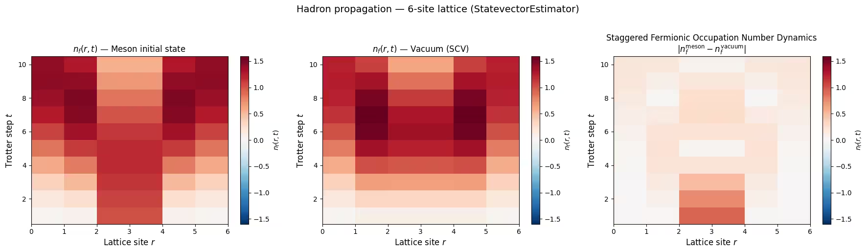
このチュートリアルはハドロン伝播をシミュレートします。強結合真空(積状態)から出発し、格子の中心に中間子を配置して時間発展させます。差分測定プロトコル — 中心の中間子ありとなしで回路を実行し、その差を取る — により、ハードウェアのノイズと境界効果の両方からコヒーレントなハドロン信号を分離します。結果として得られるのは、閉じ込められた中間子の呼吸モードに特徴的な、フェルミオン密度振動の光円錐パターンです。
要件
このチュートリアルを始める前に、以下をインストールしてください。
-
Qiskit SDK v2.0 以降(visualization サポート付き)
-
Qiskit Runtime v0.22 以降(
pip install qiskit-ibm-runtime) -
Pauli Propagation パッケージ(
pip install pauli-prop) -
NumPy (
pip install numpy) -
Matplotlib (
pip install matplotlib)
セットアップ
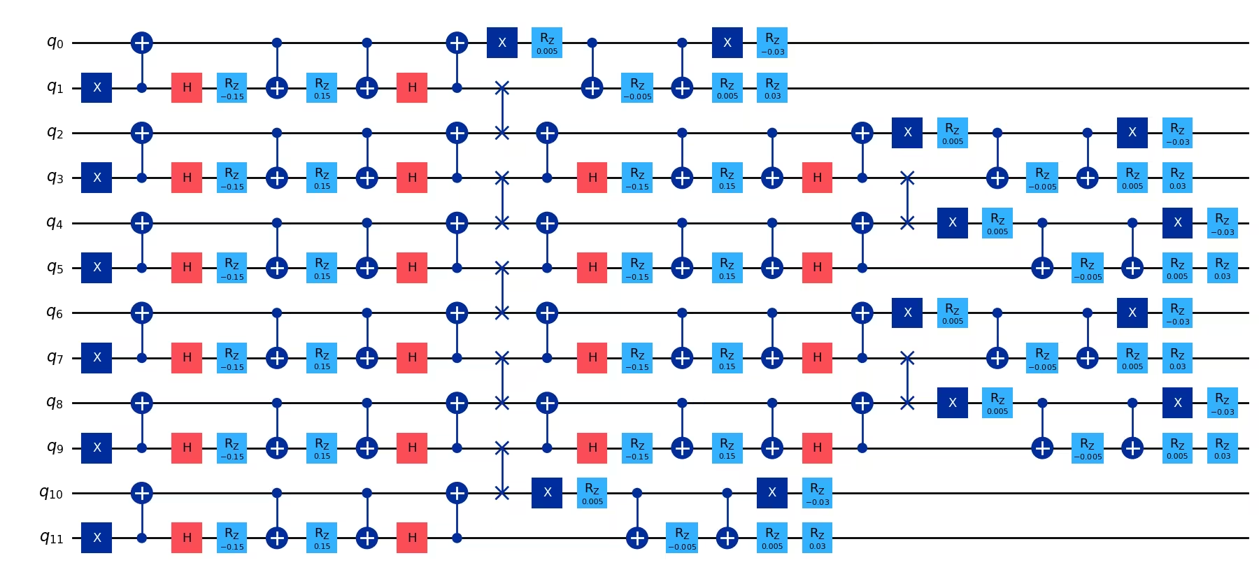
まず、必要なライブラリをインポートし、LSH 時間発展のための量子回路を構築するヘルパー関数を定義します。中心となる回路構築関数は3つあります:
-
pair_hamiltonian_circuit:隣接サイト間の近似相互作用ハミルトニアンに対する2量子ビットユニタリ を実装します。ゲート分解は次の通りです:。 -
electric_hamiltonian_circuit:各サイトにおける近似電場エネルギーに対する2量子ビットユニタリ を実装します。ゲート分解は次の通りです:。 -
construct_circuit:相互作用項、電場項、質量項を SWAP ゲートで量子ビット接続性を管理しながら重ね合わせ、完全なトロッター化回路を組み立てます。
# Added by doQumentation — required packages for this notebook
!pip install -q matplotlib numpy pauli-prop qiskit qiskit-ibm-runtime
# Import libraries

import numpy as np
import matplotlib.pyplot as plt
from matplotlib.colors import TwoSlopeNorm
from qiskit.circuit import QuantumCircuit
from qiskit.quantum_info import SparsePauliOp
from typing import Optional

import warnings

warnings.filterwarnings("ignore")
def pair_hamiltonian_circuit(c: float) -> QuantumCircuit:
    """Two-qubit unitary for the approximate interaction Hamiltonian H_I.

    Implements exp(-i * c * H_I^approx) for one pair of neighboring sites,
    where c = delta_tau * x.
    """
    qc_temp = QuantumCircuit(2)
    qc_temp.cx(1, 0)
    qc_temp.h(1)
    qc_temp.rz(-c, 1)
    qc_temp.cx(0, 1)
    qc_temp.rz(c, 1)
    qc_temp.cx(0, 1)
    qc_temp.h(1)
    qc_temp.cx(1, 0)
    return qc_temp

def electric_hamiltonian_circuit(theta: float) -> QuantumCircuit:
    """Two-qubit unitary for the approximate electric field Hamiltonian H_E.

    Implements exp(-i * theta * H_E^approx) for one lattice site,
    where theta = -delta_tau * (n_bar_l / 2 + 3/4).
    """
    qc_temp = QuantumCircuit(2)
    qc_temp.x(0)
    qc_temp.rz(theta / 2, 0)
    qc_temp.cx(0, 1)
    qc_temp.rz(-theta / 2, 1)
    qc_temp.cx(0, 1)
    qc_temp.rz(theta / 2, 1)
    qc_temp.x(0)
    return qc_temp

def construct_circuit(
    num_lattice_point: int,
    num_trotter_steps: int,
    c: float,
    theta: float,
    m: float,
    theory: Optional[int] = 2,
    barriers: Optional[bool] = False,
    measurement: Optional[bool] = False,
    add_init_state: Optional[bool] = True,
    inverse_mid: Optional[bool] = False,
) -> QuantumCircuit:
    """Construct the full Trotterized time-evolution circuit.

    Builds a circuit implementing n Trotter steps of the approximate SU(2)
    LSH Hamiltonian evolution. The qubit layout uses a zigzag ordering:
    n_i(0), n_i(1), n_o(0), n_o(1), n_i(2), n_i(3), n_o(2), n_o(3), ...
    which minimizes the number of SWAP layers needed.

    Args:
        num_lattice_point: Number of lattice sites
        (num_qubits = 2 * num_lattice_point).
        num_trotter_steps: Number of Trotter steps.
        c: Interaction parameter (delta_tau * x).
        theta: Electric field phase parameter.
        m: Mass parameter (m_tilde = delta_tau * mu).
        theory: 1 for single chain, 2 for SU(2). Default 2.
        barriers: Insert barriers between Trotter layers for
        visualization.
        measurement: Append measurements at the end.
        add_init_state: Prepare the half-filled (strong-coupling vacuum)
        initial state.
        inverse_mid: Swap the central sites
        (for differential measurement protocol).
    """
    num_qubits = theory * num_lattice_point
    qc = QuantumCircuit(num_qubits)

    if num_trotter_steps <= 0:
        return qc

    # --- Initial state preparation ---
    if add_init_state:
        i = 1
        while i < num_lattice_point:
            for j in range(theory):
                qc.x(i + j * num_lattice_point)
            i = i + 2
        if inverse_mid:
            mid_lattice_qubits = [num_qubits // 2 - 1, num_qubits // 2]
            qc.x(mid_lattice_qubits)
    else:
        i = 1
        while i < num_qubits - 1:
            qc.swap(i, i + 1)
            i = i + 4

    # --- Trotter steps ---
    for step in range(num_trotter_steps):
        if barriers:
            qc.barrier()

        # First SWAP layer (skipped at step 0 — absorbed into initial state mapping)
        if step > 0:
            i = 1
            while i < num_qubits - 1:
                qc.swap(i, i + 1)
                i = i + 4

        # First layer of pair interactions
        j = 0
        while j < num_qubits - 2:
            circ = pair_hamiltonian_circuit(c)
            qc.compose(circ, [j, j + 1], inplace=True)
            j = j + 2
        if num_lattice_point % 2 == 0:
            circ = pair_hamiltonian_circuit(c)
            qc.compose(circ, [j, j + 1], inplace=True)

        # Second SWAP layer
        i = 1
        while i < num_qubits - 1:
            qc.swap(i, i + 1)
            i = i + theory

        # Second layer of pair interactions
        j = 2
        while j < num_qubits - 3:
            circ = pair_hamiltonian_circuit(c)
            qc.compose(circ, [j, j + 1], inplace=True)
            j = j + 2
        if num_lattice_point % 2 != 0:
            circ = pair_hamiltonian_circuit(c)
            qc.compose(circ, [j, j + 1], inplace=True)

        # Third SWAP layer
        i = 3
        while i < num_qubits - 1:
            qc.swap(i, i + 1)
            i = i + 2 * theory

        # Electric field term
        if theta != 0:
            e_circ = electric_hamiltonian_circuit(theta)
            for j in range(num_lattice_point):
                qc.compose(e_circ, [2 * j, 2 * j + 1], inplace=True)

        # Mass term: Rz(-m_tilde) for even sites, Rz(m_tilde) for odd sites
        for q in range(num_qubits):
            if q % 2 == 0:
                qc.rz(-1 * m, q)
            else:
                qc.rz(m, q)

    if measurement:
        qc.measure_all()

    return qc
def get_probabilities(expval: float):
    """Convert a Z-expectation value to site occupation probability.

    Since <Z> = p(0) - p(1), the occupation probability is p(1) = (1 - <Z>) / 2.
    """
    p1 = round((1 - expval) / 2, 3)
    return p1

def get_number(expval_data, num_lattice_point):
    """Convert raw Z-expectation values to staggered fermion number n_f at each site.

    n_f(r) = n_i(r) + n_o(r)           for even r
    n_f(r) = 2 - [n_i(r) + n_o(r)]     for odd r

    The two qubits per site encode (n_i, n_o), and occupation probabilities
    give us <n_i> and <n_o>.
    """
    N = []
    for expvals in expval_data:
        Pstep = [get_probabilities(expval) for expval in expvals]
        Nstep = []
        for k in range(num_lattice_point):
            val = Pstep[2 * k] + Pstep[2 * k + 1]
            a = 2 * (k % 2) + (1 - 2 * (k % 2)) * val
            Nstep.append(float(a))
        N.append(Nstep)
    return N

def calculate_difference(N, N_mid, num_lattice_point):
    """Differential measurement protocol: |n_f(meson) - n_f(vacuum)|.

    Subtracting the vacuum (SCV) evolution from the meson evolution
    isolates the coherent hadron signal from symmetric noise and boundary effects.
    """
    N_diff = []
    for i in range(len(N)):
        Nstep_diff = []
        for j in range(num_lattice_point):
            Nstep_diff.append(abs(N[i][j] - N_mid[i][j]))
        N_diff.append(Nstep_diff)
    return N_diff
小規模シミュレータの例
まず、6サイトの格子(12量子ビット)を使用して小規模でワークフローを実演し、ハードウェア上で実行する前に回路構築を検証し、物理的な観測量を理解できるようにします。
ステップ1:古典的な入力を量子問題にマッピングする
論文で研究された弱結合領域(、)に一致する物理パラメータを定義します。導出される回路パラメータは以下の通りです:
-
(相互作用パラメータ)
-
(電場位相)
-
(質量パラメータ)
各トロッター・ステップ数について、2つの回路を構築します。1つは中心に中間子を初期化する回路(inverse_mid=True)、もう1つは強結合真空を準備する回路(inverse_mid=False)です。差分測定プロトコルは、真空の発展を差し引くことでハドロン信号を分離します。
# Physical / circuit parameters
num_lattice_point = 6  # 6 lattice sites -> 12 qubits for SU(2)
num_qubits = 2 * num_lattice_point
c = 0.15  # delta_tau * x
theta = 0.01  # electric field phase
m = 0.03  # m_tilde = delta_tau * mu
trotter_steps = range(1, 11)  # 10 Trotter steps

print(f"Lattice sites: {num_lattice_point}, Qubits: {num_qubits}")
print(f"Parameters: c={c}, theta={theta}, m_tilde={m}")
Lattice sites: 6, Qubits: 12
Parameters: c=0.15, theta=0.01, m_tilde=0.03
# Build circuits: meson initial state and vacuum (SCV) initial state
circuits_mid = [
    construct_circuit(
        num_lattice_point,
        d,
        c,
        theta,
        m,
        barriers=False,
        measurement=False,
        add_init_state=True,
        inverse_mid=True,
    )
    for d in trotter_steps
]

circuits = [
    construct_circuit(
        num_lattice_point,
        d,
        c,
        theta,
        m,
        barriers=False,
        measurement=False,
        add_init_state=True,
        inverse_mid=False,
    )
    for d in trotter_steps
]

# Visualize a single Trotter step
print(
    f"Circuit for 1 Trotter step: {circuits[0].num_qubits} qubits, depth {circuits[0].depth()}"
)
circuits[0].draw("mpl", fold=-1)
Circuit for 1 Trotter step: 12 qubits, depth 26
ステップ2:量子ハードウェア実行のために問題を最適化する
観測量を定義します:すべての量子ビットに対する単一量子ビット 測定です。 から占有確率、さらに各格子サイト におけるスタッガード・フェルミオン数 を抽出できます。
# Z observable on each qubit
observables = [
    SparsePauliOp("I" * i + "Z" + "I" * (num_qubits - i - 1))
    for i in range(num_qubits)
]

print(f"Number of observables: {len(observables)}")
Number of observables: 12
ステップ3:Qiskit プリミティブを使用して実行する
小規模での正確なノイズなしシミュレーションには StatevectorEstimator を使用します。
from qiskit.primitives import StatevectorEstimator

estimator = StatevectorEstimator()

# Run meson circuits
pubs_mid = [(circuit, observables) for circuit in circuits_mid]
result_mid = estimator.run(pubs_mid).result()

# Run vacuum (SCV) circuits
pubs = [(circuit, observables) for circuit in circuits]
result = estimator.run(pubs).result()

# Extract expectation values
raw_expvals_mid = [
    result_mid[i].data.evs[::-1] for i in range(len(circuits_mid))
]
raw_expvals = [result[i].data.evs[::-1] for i in range(len(circuits))]

print(f"Computed expectation values for {len(raw_expvals)} Trotter steps")
Computed expectation values for 10 Trotter steps
ステップ4:後処理を行い、望ましい古典形式で結果を返す
期待値をスタッガード・フェルミオン数 に変換し、差分測定プロトコル(中間子 真空)を適用して、ハドロン伝播ヒートマップを生成します。これは、参照論文の図3の構造を再現します:x軸に格子サイト 、y軸にトロッター・ステップ(時間)、そして をカラースケールとして表します。
# Compute fermion numbers
N_mid_sim = get_number(raw_expvals_mid, num_lattice_point)
N_sim = get_number(raw_expvals, num_lattice_point)
N_diff_sim = calculate_difference(N_mid_sim, N_sim, num_lattice_point)

# --- Reproduce Figure 3 style: Staggered Fermionic Occupation Number Dynamics ---
fig, axes = plt.subplots(1, 3, figsize=(18, 5))

# Convert to numpy arrays for plotting
N_mid_arr = np.array(N_mid_sim)
N_arr = np.array(N_sim)
N_diff_arr = np.array(N_diff_sim)

# Color scheme
vmax = max(max(sublist) for sublist in N_arr)
vmin = -vmax

# Meson evolution
norm1 = TwoSlopeNorm(vmin=vmin, vcenter=0, vmax=vmax)
im0 = axes[0].imshow(
    N_mid_arr,
    aspect="auto",
    origin="lower",
    cmap="RdBu_r",
    norm=norm1,
    extent=[0, num_lattice_point, 0.5, len(trotter_steps) + 0.5],
)
axes[0].set_xlabel("Lattice site $r$", fontsize=12)
axes[0].set_ylabel("Trotter step $t$", fontsize=12)
axes[0].set_title("$n_f(r,t)$ — Meson initial state", fontsize=12)
plt.colorbar(im0, ax=axes[0], label="$n_f(r,t)$")

# Vacuum (SCV) evolution
im1 = axes[1].imshow(
    N_arr,
    aspect="auto",
    origin="lower",
    cmap="RdBu_r",
    norm=norm1,
    extent=[0, num_lattice_point, 0.5, len(trotter_steps) + 0.5],
)
axes[1].set_xlabel("Lattice site $r$", fontsize=12)
axes[1].set_ylabel("Trotter step $t$", fontsize=12)
axes[1].set_title("$n_f(r,t)$ — Vacuum (SCV)", fontsize=12)
plt.colorbar(im1, ax=axes[1], label="$n_f(r,t)$")

# Differential: meson - vacuum
norm2 = TwoSlopeNorm(vmin=vmin, vcenter=0, vmax=vmax)
im2 = axes[2].imshow(
    N_diff_arr,
    aspect="auto",
    origin="lower",
    cmap="RdBu_r",
    norm=norm2,
    extent=[0, num_lattice_point, 0.5, len(trotter_steps) + 0.5],
)
axes[2].set_xlabel("Lattice site $r$", fontsize=12)
axes[2].set_ylabel("Trotter step $t$", fontsize=12)
axes[2].set_title(
    "Staggered Fermionic Occupation Number Dynamics\n$|n_f^{\\mathrm{meson}} - n_f^{\\mathrm{vacuum}}|$",
    fontsize=12,
)
plt.colorbar(im2, ax=axes[2], label="$n_f(r,t)$")

plt.suptitle(
    f"Hadron propagation — {num_lattice_point}-site lattice (StatevectorEstimator)",
    fontsize=14,
    y=1.02,
)
plt.tight_layout()
plt.show()
大規模ハードウェアの例
ここでは、IBM Quantum ハードウェア上で30サイトの格子(60量子ビット)へとスケールアップします。この規模では、10トロッター・ステップの回路は3400を超える2量子ビットゲートと14,000個の単一量子ビットゲートで構成されます。
ステップ1〜4(1つのコードブロックにまとめたもの)
ハードウェア・ワークフローの主な特徴:
-
中間子回路と真空回路のための10トロッター・ステップ(ドリフトを最小化するためにインターリーブ)
-
optimization_level=1でのトランスパイル — 回路レイアウトはすでにデバイス・トポロジー(線形鎖)と同型であるため、ルーティング用の SWAP は不要です。トランスパイラーは、低ノイズな物理量子ビットの鎖を選択し、ゲートをネイティブ・ゲートセットに分解するためだけに使用されます。 -
TREX 読み出しエラー抑制とパウリ・ツイリングを伴う
EstimatorV2 -
すべてのジョブをまとめて送信するための
Batchセッション
# -------------------------Step 1: Define parameters & build circuits-------------------------

from qiskit_ibm_runtime import QiskitRuntimeService
from qiskit.transpiler.preset_passmanagers import generate_preset_pass_manager
from qiskit_ibm_runtime import EstimatorV2, Batch
from qiskit_ibm_runtime.options import (
    EstimatorOptions,
    ResilienceOptionsV2,
    TwirlingOptions,
    DynamicalDecouplingOptions,
)

service = QiskitRuntimeService()

num_lattice_point_hw = 30
num_qubits_hw = 2 * num_lattice_point_hw  # 60 qubits
c_hw = 0.15
theta_hw = 0.01
m_hw = 0.03
trotter_steps_hw = range(1, 11)  # 10 Trotter steps

# Build meson and vacuum circuits
circuits_mid_hw = [
    construct_circuit(
        num_lattice_point_hw,
        d,
        c_hw,
        theta_hw,
        m_hw,
        barriers=False,
        measurement=False,
        add_init_state=True,
        inverse_mid=True,
    )
    for d in trotter_steps_hw
]

circuits_hw = [
    construct_circuit(
        num_lattice_point_hw,
        d,
        c_hw,
        theta_hw,
        m_hw,
        barriers=False,
        measurement=False,
        add_init_state=True,
        inverse_mid=False,
    )
    for d in trotter_steps_hw
]

print(f"Built {len(circuits_hw)} circuit pairs for {num_qubits_hw} qubits")

# -------------------------Step 2: Transpile for hardware-------------------------
# The circuit topology is a linear chain, isomorphic to the device topology.
# We use optimization_level=1 since no routing SWAPs are needed — the transpiler
# only needs to select a low-noise qubit chain and decompose to native gates.

backend = service.backend("ibm_boston")

layout = [
    140,
    141,
    142,
    143,
    136,
    123,
    122,
    121,
    116,
    101,
    102,
    103,
    96,
    83,
    82,
    81,
    76,
    61,
    62,
    63,
    64,
    65,
    66,
    67,
    68,
    69,
    78,
    89,
    88,
    87,
    97,
    107,
    106,
    105,
    117,
    125,
    126,
    127,
    137,
    147,
    148,
    149,
    150,
    151,
    152,
    153,
    154,
    155,
    139,
    135,
    134,
    133,
    132,
    131,
    130,
    129,
    118,
    109,
    110,
    111,
]

pm = generate_preset_pass_manager(
    optimization_level=1, backend=backend, initial_layout=layout
)

isa_circuits_mid = pm.run(circuits_mid_hw)
isa_circuits = pm.run(circuits_hw)

print(f"Transpiled circuits. Example depth: {isa_circuits[0].depth()}")

# Define and layout-map observables
observables_hw = [
    SparsePauliOp("I" * i + "Z" + "I" * (num_qubits_hw - i - 1))
    for i in range(num_qubits_hw)
]

isa_observables_mid = [
    [obs.apply_layout(isa_circuits_mid[i].layout) for obs in observables_hw]
    for i in range(len(isa_circuits_mid))
]
isa_observables = [
    [obs.apply_layout(isa_circuits[i].layout) for obs in observables_hw]
    for i in range(len(isa_circuits))
]

# Build PUBs — interleave meson and vacuum for each Trotter step
isa_pubs_mid = [
    (circ, obs) for circ, obs in zip(isa_circuits_mid, isa_observables_mid)
]
isa_pubs = [(circ, obs) for circ, obs in zip(isa_circuits, isa_observables)]

pubs_to_execute = [
    [isa_pubs_mid[i], isa_pubs[i]] for i in range(len(isa_pubs))
]

# -------------------------Step 3: Execute on hardware-------------------------

twirling_options = TwirlingOptions(
    enable_gates=True,
    enable_measure=True,
    shots_per_randomization="auto",
    strategy="active-circuit",
)

resilience_options = ResilienceOptionsV2(
    measure_mitigation=True,  # TREX readout error mitigation
    zne_mitigation=False,  # ZNE turned off
)

dd_options = DynamicalDecouplingOptions(
    enable=False  # Circuit is sufficiently dense
)

options = EstimatorOptions(
    resilience=resilience_options,
    twirling=twirling_options,
    dynamical_decoupling=dd_options,
    default_shots=10_000,
)

ids = []
with Batch(backend=backend) as batch:
    for idx, pub in enumerate(pubs_to_execute):
        print(f"Submitting job for Trotter step {idx + 1}")
        estimator = EstimatorV2(mode=batch, options=options)
        estimator.skip_transpilation = True
        job = estimator.run(pub)
        ids.append(job.job_id())
    batch_id = batch.session_id

job_info = {"ids": ids, "batch_id": batch_id}
print(f"Submitted {len(ids)} jobs. Batch ID: {batch_id}")
print(ids)
# -------------------------Step 4: Post-process results-------------------------

jobs = [service.job(job_id) for job_id in ids]
results = [job.result() for job in jobs]

# Extract expectation values (index 0 = meson, index 1 = vacuum)
raw_expvals_mid_hw = [result[0].data.evs[::-1] for result in results]
raw_expvals_hw = [result[1].data.evs[::-1] for result in results]

# Compute fermion numbers and differential
N_mid_hw = get_number(raw_expvals_mid_hw, num_lattice_point_hw)
N_hw = get_number(raw_expvals_hw, num_lattice_point_hw)
N_diff_hw = calculate_difference(N_mid_hw, N_hw, num_lattice_point_hw)
N_diff_hw_arr = np.array(N_diff_hw)

fig, ax = plt.subplots(figsize=(10, 6))
vmax = np.abs(N_hw).max()
vmin = -vmax
norm = TwoSlopeNorm(vmin=vmin, vcenter=0, vmax=vmax)
im = ax.imshow(
    N_diff_hw_arr,
    aspect="auto",
    origin="lower",
    cmap="RdBu_r",
    norm=norm,
    extent=[0, 8, 0.5, len(trotter_steps_hw) + 0.5],
)
ax.set_xlabel("Lattice site $r$", fontsize=13)
ax.set_ylabel("Trotter step $t$", fontsize=13)
ax.set_title(
    "Staggered Fermionic Occupation Number Dynamics\nQuantum Simulation on IBM Hardware — 30-site lattice (60 qubits)",
    fontsize=13,
)
cbar = plt.colorbar(im, ax=ax)
cbar.set_label("$n_f(r,t)$", fontsize=12)
plt.tight_layout()
plt.show()

Pauli Propagation による古典的ベンチマーク
パウリ伝播法(PPM)は、ハイゼンベルク描像で測定観測量を回路を通じて逆伝播させることにより、量子回路のノイズなし古典シミュレーションを提供します。クリフォード層(CNOT、H、S、X ゲート)の下では、パウリ演算子は項数を増やすことなく他のパウリ演算子に写像されます。非クリフォード層(回路中の ゲート)は分岐を引き起こす可能性があり — 最悪の場合、項数が2倍になります — が、多くの分岐は係数が小さいため打ち切ることができます。
pauli-prop を用いたワークフローは以下の通りです:
-
分割:
evolve_through_cliffordsを使用して、回路をクリフォード部分と非クリフォード部分に分割します。 -
伝播:
propagate_through_circuitを使用して、各観測量を非クリフォード部分を通じて伝播させ、最大max_terms個のパウリ項を保持し、打ち切りしきい値atolを下回る係数を持つ項を破棄します。 -
発展:Qiskit 組み込みのクリフォード・サポートを使用して、結果をクリフォード部分を通じて発展させます。
-
抽出:対角パウリ項( と のみを含む)の係数を合計することで、期待値を抽出します。
打ち切りしきい値
propagate_through_circuit の atol パラメータは、小さなパウリ分岐をどれだけ積極的に刈り込むかを制御します。非常に厳しいしきい値(例えば 1e-12)はほぼすべての分岐を保持し、正確な結果を与えますが、シミュレーション時間は回路深さとともに急激に増加します。論文における120量子ビットのシミュレーションでは、デフォルト設定で約8.5時間かかりました。しきい値を上げる(例えば 1e-6 や 1e-3 にする)と、その値を下回る係数を持つ項が破棄され、追跡される項の数が劇的に減少し、計算が高速化されます。トレードオフは、小さく制御可能な近似誤差であり、異なるしきい値での結果を比較することで検証できます。
import time
from pauli_prop import evolve_through_cliffords, propagate_through_circuit

# ── PPM Configuration ──
# Truncation threshold: controls the speed/accuracy trade-off.
PPM_THRESHOLD = 1e-3

# Maximum Pauli terms to track per observable (hard cap on memory/time)
PPM_MAX_TERMS = 66_000

print(f"PPM settings: atol={PPM_THRESHOLD}, max_terms={PPM_MAX_TERMS}")

# We propagate each single-qubit Z observable through each circuit.
# For PPM, we work with the un-transpiled circuits (ideal noiseless simulation).

observables_pp = [
    SparsePauliOp("I" * i + "Z" + "I" * (num_qubits_hw - i - 1))
    for i in range(num_qubits_hw)
]

def ppm_expectation_values(
    circuit, observables, max_terms=PPM_MAX_TERMS, atol=PPM_THRESHOLD
):
    """Compute expectation values of single-qubit Z observables
    via Pauli propagation.

    Args:
        circuit: The quantum circuit to simulate.
        observables: List of single-qubit Z observables.
        max_terms: Maximum number of Pauli terms to retain (hard cap).
        atol: Absolute tolerance — Pauli terms with coefficients below this
              value are discarded during propagation. Larger values give
              faster simulation at the cost of approximation accuracy.
    """
    circuit = circuit.decompose(["swap"])  # decompose SWAPs into 3 CX gates
    cliff, non_cliff = evolve_through_cliffords(circuit)

    evs = []
    for obs in observables:
        evolved_obs = propagate_through_circuit(
            obs, non_cliff, max_terms=max_terms, atol=atol, frame="h"
        )[0]
        evolved_obs.paulis = evolved_obs.paulis.evolve(cliff, frame="h")
        diagonal_mask = ~evolved_obs.paulis.x.any(axis=1)
        ev = float(evolved_obs.coeffs[diagonal_mask].sum().real)
        evs.append(ev)
    return np.array(evs)

# Run PPM for each Trotter step and record wall-clock time
pp_expvals_mid = []
pp_expvals = []
pp_times = []

for idx, d in enumerate(trotter_steps_hw):
    t_start = time.perf_counter()

    # Meson circuit
    evs_mid = ppm_expectation_values(circuits_mid_hw[idx], observables_pp)

    # Vacuum circuit
    evs_vac = ppm_expectation_values(circuits_hw[idx], observables_pp)

    elapsed = time.perf_counter() - t_start
    pp_times.append(elapsed)

    pp_expvals_mid.append(evs_mid[::-1])
    pp_expvals.append(evs_vac[::-1])

    print(f"Trotter step {d:2d}: {elapsed:.1f} s")

print(f"\nTotal PPM simulation time: {sum(pp_times):.1f} s")
print(f"Truncation threshold used: {PPM_THRESHOLD}")
PPM settings: atol=0.001, max_terms=66000
Trotter step  1: 5.0 s
Trotter step  2: 7.5 s
Trotter step  3: 11.2 s
Trotter step  4: 14.7 s
Trotter step  5: 18.3 s
Trotter step  6: 22.1 s
Trotter step  7: 25.6 s
Trotter step  8: 29.4 s
Trotter step  9: 33.2 s
Trotter step 10: 36.6 s

Total PPM simulation time: 203.6 s
Truncation threshold used: 0.001
# --- PPM simulation time vs. Trotter steps ---
fig, ax = plt.subplots(figsize=(8, 5))
ax.plot(
    list(trotter_steps_hw),
    pp_times,
    "o-",
    color="tab:blue",
    linewidth=2,
    markersize=6,
)
ax.set_xlabel("Trotter step", fontsize=13)
ax.set_ylabel("Wall-clock time (s)", fontsize=13)
ax.set_title(
    "Pauli Propagation simulation time vs. Trotter steps\n(30-site lattice, 60 qubits)",
    fontsize=13,
)
ax.grid(True, alpha=0.3)
plt.tight_layout()
plt.show()

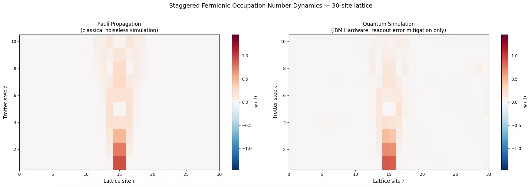
# --- PPM heatmap and comparison with hardware ---
N_mid_pp = get_number(pp_expvals_mid, num_lattice_point_hw)
N_pp = get_number(pp_expvals, num_lattice_point_hw)
N_diff_pp = calculate_difference(N_mid_pp, N_pp, num_lattice_point_hw)

N_diff_pp_arr = np.array(N_diff_pp)

fig, axes = plt.subplots(1, 2, figsize=(18, 6))
vmax = np.abs(N_hw).max()
vmin = -vmax
norm = TwoSlopeNorm(vmin=vmin, vcenter=0, vmax=vmax)

# PPM result
im0 = axes[0].imshow(
    N_diff_pp_arr,
    aspect="auto",
    origin="lower",
    cmap="RdBu_r",
    norm=norm,
    extent=[0, num_lattice_point_hw, 0.5, len(trotter_steps_hw) + 0.5],
)
axes[0].set_xlabel("Lattice site $r$", fontsize=12)
axes[0].set_ylabel("Trotter step $t$", fontsize=12)
axes[0].set_title(
    "Pauli Propagation\n(classical noiseless simulation)", fontsize=12
)
plt.colorbar(im0, ax=axes[0], label="$n_f(r,t)$")

# Hardware result
im1 = axes[1].imshow(
    N_diff_hw_arr,
    aspect="auto",
    origin="lower",
    cmap="RdBu_r",
    norm=norm,
    extent=[0, num_lattice_point_hw, 0.5, len(trotter_steps_hw) + 0.5],
)
axes[1].set_xlabel("Lattice site $r$", fontsize=12)
axes[1].set_ylabel("Trotter step $t$", fontsize=12)
axes[1].set_title(
    "Quantum Simulation\n(IBM Hardware, readout error mitigation only)",
    fontsize=12,
)
plt.colorbar(im1, ax=axes[1], label="$n_f(r,t)$")

plt.suptitle(
    "Staggered Fermionic Occupation Number Dynamics — 30-site lattice",
    fontsize=14,
    y=1.02,
)
plt.tight_layout()
plt.show()
次のステップ
この内容に興味を持った方は、以下の資料を調べてみることをご検討ください。
-
Qiskit Estimator プリミティブのドキュメント — エラー抑制オプションの設定方法の詳細について
-
エラー抑制と抑圧の手法 — TREX、ZNE、その他の抑制手法について学ぶために
-
Qiskit Pauli Propagation(pauli-prop) — パウリ逆伝播による Rust 高速化された古典シミュレーション
参考文献
[1] 原論文:Ilčić, Majumdar, Mathew et al. 「Observation of Robust and Coherent Non-Abelian Hadron Dynamics on Noisy Quantum Processors」arXiv:2602.18080 (2026)