確率的エラー増幅によるユーティリティスケールのエラー軽減

使用量の目安: Heron r2 プロセッサで16分（注意: これは目安です。実際の実行時間は異なる場合があります。）

背景

このチュートリアルでは、Qiskit Runtime を使用して、確率的エラー増幅（PEA）を用いたゼロノイズ外挿（ZNE）の実験的バージョンによるユーティリティスケールのエラー軽減実験を実行する方法を説明します。

参考文献: Y. Kim et al. Evidence for the utility of quantum computing before fault tolerance. Nature 618.7965 (2023)

ゼロノイズ外挿（ZNE）

ゼロノイズ外挿（ZNE）は、回路実行中の未知のノイズの影響を、既知の方法でスケーリングできることを利用して除去するエラー軽減技術です。

この手法は、期待値がノイズに対して既知の関数でスケーリングすることを仮定しています。

$$\langle A(\lambda) \rangle = \langle A(0) \rangle + \sum_{k=0}^{m} a_k \lambda^k + R$$

ここで $\lambda$ はノイズの強度をパラメータ化しており、増幅することができます。 ZNE は以下の手順で実装できます。

1. 複数のノイズ係数 $\lambda_1, \lambda_2, ...$ に対して回路のノイズを増幅します
2. すべてのノイズ増幅回路を実行して $\langle A(\lambda_1)\rangle, ...$ を測定します
3. ゼロノイズ極限 $\langle A(0)\rangle$ に外挿します

ZNE のノイズ増幅

ZNE を正しく実装する上での主な課題は、期待値におけるノイズの正確なモデルを持ち、既知の方法でノイズを増幅することです。

ZNE のエラー増幅を実装する一般的な方法は3つあります。

パルス伸長	ゲート折り畳み	確率的エラー増幅
キャリブレーションによりパルス持続時間をスケーリング	恒等サイクルでゲートを繰り返す $U\mapsto U(U^{-1}U)^{\lambda-1}/2$	パウリチャネルのサンプリングによりノイズを追加
Kandala et al. Nature (2019)	Shultz et al. PRA (2022)	Li & Benjamin PRX (2017)
ユーティリティスケールの実験において、確率的エラー増幅（PEA）が最も魅力的です。

• パルス伸長は、ゲートノイズが持続時間に比例することを仮定しますが、通常これは正しくありません。また、キャリブレーションにもコストがかかります。
• ゲート折り畳みは大きなストレッチ係数を必要とし、実行可能な回路の深さを大幅に制限します。
• PEA は、ネイティブノイズ係数（$\lambda=1$）で実行可能な任意の回路に適用できますが、ノイズモデルの学習が必要です。

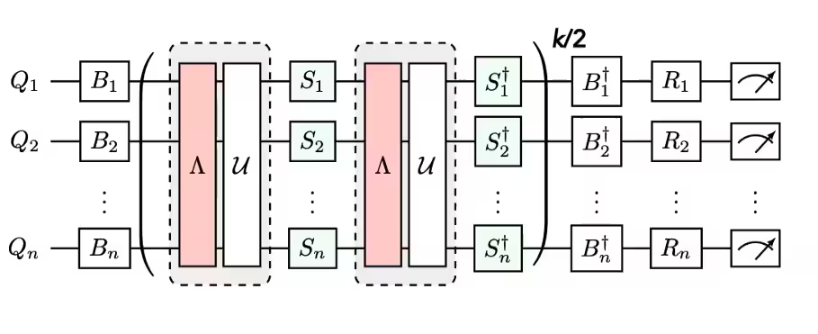
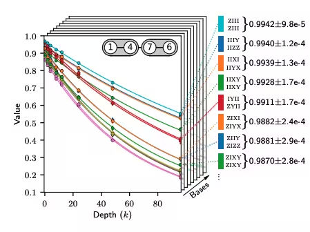
PEA のためのノイズモデル学習

PEA は確率的エラーキャンセレーション（PEC）と同じ層ベースのノイズモデルを仮定しますが、回路ノイズに対して指数的にスケーリングするサンプリングオーバーヘッドを回避します。

ステップ 1	ステップ 2	ステップ 3
2量子ビットゲートの層にパウリツイルを適用	層の恒等ペアを繰り返してノイズを学習	忠実度（各ノイズチャネルのエラー）を導出

参考文献: E. van den Berg, Z. Minev, A. Kandala, and K. Temme, Probabilistic error cancellation with sparse Pauli-Lindblad models on noisy quantum processors arXiv:2201.09866

要件

このチュートリアルを開始する前に、以下がインストールされていることを確認してください。

• Qiskit SDK v1.0 以降（visualization サポート付き）
• Qiskit Runtime v0.22 以降（pip install qiskit-ibm-runtime）

セットアップ

from __future__ import annotations
from collections.abc import Sequence
from collections import defaultdict
import numpy as np
import rustworkx
import matplotlib.pyplot as plt

from qiskit.circuit import QuantumCircuit, Parameter
from qiskit.circuit.library import CXGate, CZGate, ECRGate
from qiskit.providers import Backend
from qiskit.visualization import plot_error_map
from qiskit.transpiler.preset_passmanagers import generate_preset_pass_manager
from qiskit.quantum_info import SparsePauliOp
from qiskit.primitives import PubResult

from qiskit_ibm_runtime import QiskitRuntimeService
from qiskit_ibm_runtime import EstimatorV2 as Estimator

ステップ 1: 古典的な入力を量子問題にマッピングする

パラメータ化されたイジングモデル回路の作成

まず、実行するバックエンドを選択します。このデモンストレーションでは127量子ビットのバックエンドで実行しますが、利用可能な任意のバックエンドに変更することができます。

service = QiskitRuntimeService()
backend = service.least_busy(
    operational=True, simulator=False, min_num_qubits=127
)
backend

<IBMBackend('ibm_kingston')>

回路構築のためのヘルパー関数

次に、バックエンドのトポロジーに準拠した2次元横磁場イジングモデルのトロッター化された時間発展のための回路を構築するヘルパー関数を作成します。

"""Trotter circuit generation"""

def remove_qubit_couplings(
    couplings: Sequence[tuple[int, int]], qubits: Sequence[int] | None = None
) -> list[tuple[int, int]]:
    """Remove qubits from a coupling list.

    Args:
        couplings: A sequence of qubit couplings.
        qubits: Optional, the qubits to remove.

    Returns:
        The input couplings with the specified qubits removed.
    """
    if qubits is None:
        return couplings
    qubits = set(qubits)
    return [edge for edge in couplings if not qubits.intersection(edge)]

def coupling_qubits(
    *couplings: Sequence[tuple[int, int]],
    allowed_qubits: Sequence[int] | None = None,
) -> list[int]:
    """Return a sorted list of all qubits involved in one or more couplings lists.

    Args:
        couplings: one or more coupling lists.
        allowed_qubits: Optional, the allowed qubits to include. If None all
            qubits are allowed.

    Returns:
        The intersection of all qubits in the couplings and the allowed qubits.
    """
    qubits = set()
    for edges in couplings:
        for edge in edges:
            qubits.update(edge)
    if allowed_qubits is not None:
        qubits = qubits.intersection(allowed_qubits)
    return list(qubits)

def construct_layer_couplings(
    backend: Backend,
) -> list[list[tuple[int, int]]]:
    """Separate a coupling map into disjoint 2-qubit gate layers.

    Args:
        backend: A backend to construct layer couplings for.

    Returns:
        A list of disjoint layers of directed couplings for the input coupling map.
    """
    coupling_graph = backend.coupling_map.graph.to_undirected(
        multigraph=False
    )
    edge_coloring = rustworkx.graph_bipartite_edge_color(coupling_graph)

    layers = defaultdict(list)
    for edge_idx, color in edge_coloring.items():
        layers[color].append(
            coupling_graph.get_edge_endpoints_by_index(edge_idx)
        )
    layers = [sorted(layers[i]) for i in sorted(layers.keys())]

    return layers

def entangling_layer(
    gate_2q: str,
    couplings: Sequence[tuple[int, int]],
    qubits: Sequence[int] | None = None,
) -> QuantumCircuit:
    """Generating a entangling layer for the specified couplings.

    This corresponds to a Trotter layer for a ZZ Ising term with angle Pi/2.

    Args:
        gate_2q: The 2-qubit basis gate for the layer, should be "cx", "cz", or "ecr".
        couplings: A sequence of qubit couplings to add CX gates to.
        qubits: Optional, the physical qubits for the layer. Any couplings involving
            qubits not in this list will be removed. If None the range up to the largest
            qubit in the couplings will be used.

    Returns:
        The QuantumCircuit for the entangling layer.
    """
    # Get qubits and convert to set to order
    if qubits is None:
        qubits = range(1 + max(coupling_qubits(couplings)))
    qubits = set(qubits)

    # Mapping of physical qubit to virtual qubit
    qubit_mapping = {q: i for i, q in enumerate(qubits)}

    # Convert couplings to indices for virtual qubits
    indices = [
        [qubit_mapping[i] for i in edge]
        for edge in couplings
        if qubits.issuperset(edge)
    ]

    # Layer circuit on virtual qubits
    circuit = QuantumCircuit(len(qubits))

    # Get 2-qubit basis gate and pre and post rotation circuits
    gate2q = None
    pre = QuantumCircuit(2)
    post = QuantumCircuit(2)

    if gate_2q == "cx":
        gate2q = CXGate()
        # Pre-rotation
        pre.sdg(0)
        pre.z(1)
        pre.sx(1)
        pre.s(1)
        # Post-rotation
        post.sdg(1)
        post.sxdg(1)
        post.s(1)
    elif gate_2q == "ecr":
        gate2q = ECRGate()
        # Pre-rotation
        pre.z(0)
        pre.s(1)
        pre.sx(1)
        pre.s(1)
        # Post-rotation
        post.x(0)
        post.sdg(1)
        post.sxdg(1)
        post.s(1)
    elif gate_2q == "cz":
        gate2q = CZGate()
        # Identity pre-rotation
        # Post-rotation
        post.sdg([0, 1])
    else:
        raise ValueError(
            f"Invalid 2-qubit basis gate {gate_2q}, should be 'cx', 'cz', or 'ecr'"
        )

    # Add 1Q pre-rotations
    for inds in indices:
        circuit.compose(pre, qubits=inds, inplace=True)

    # Use barriers around 2-qubit basis gate to specify a layer for PEA noise learning
    circuit.barrier()
    for inds in indices:
        circuit.append(gate2q, (inds[0], inds[1]))
    circuit.barrier()

    # Add 1Q post-rotations after barrier
    for inds in indices:
        circuit.compose(post, qubits=inds, inplace=True)

    # Add physical qubits as metadata
    circuit.metadata["physical_qubits"] = tuple(qubits)

    return circuit

def trotter_circuit(
    theta: Parameter | float,
    layer_couplings: Sequence[Sequence[tuple[int, int]]],
    num_steps: int,
    gate_2q: str | None = "cx",
    backend: Backend | None = None,
    qubits: Sequence[int] | None = None,
) -> QuantumCircuit:
    """Generate a Trotter circuit for the 2D Ising

    Args:
        theta: The angle parameter for X.
        layer_couplings: A list of couplings for each entangling layer.
        num_steps: the number of Trotter steps.
        gate_2q: The 2-qubit basis gate to use in entangling layers.
            Can be "cx", "cz", "ecr", or None if a backend is provided.
        backend: A backend to get the 2-qubit basis gate from, if provided
            will override the basis_gate field.
        qubits: Optional, the allowed physical qubits to truncate the
            couplings to. If None the range up to the largest
            qubit in the couplings will be used.

    Returns:
        The Trotter circuit.
    """
    if backend is not None:
        try:
            basis_gates = backend.configuration().basis_gates
        except AttributeError:
            basis_gates = backend.basis_gates
        for gate in ["cx", "cz", "ecr"]:
            if gate in basis_gates:
                gate_2q = gate
                break

    # If no qubits, get the largest qubit from all layers and
    # specify the range so the same one is used for all layers.
    if qubits is None:
        qubits = range(1 + max(coupling_qubits(layer_couplings)))

    # Generate the entangling layers
    layers = [
        entangling_layer(gate_2q, couplings, qubits=qubits)
        for couplings in layer_couplings
    ]

    # Construct the circuit for a single Trotter step
    num_qubits = len(qubits)
    trotter_step = QuantumCircuit(num_qubits)
    trotter_step.rx(theta, range(num_qubits))
    for layer in layers:
        trotter_step.compose(layer, range(num_qubits), inplace=True)

    # Construct the circuit for the specified number of Trotter steps
    circuit = QuantumCircuit(num_qubits)
    for _ in range(num_steps):
        circuit.rx(theta, range(num_qubits))
        for layer in layers:
            circuit.compose(layer, range(num_qubits), inplace=True)

    circuit.metadata["physical_qubits"] = tuple(qubits)
    return circuit

エンタングリング層の結合の定義

トロッター化されたイジングシミュレーションを実装するために、デバイスの2量子ビットゲート結合の3つの層を定義します。これらは各トロッターステップで繰り返されます。これにより、エラー軽減を実装するためにノイズを学習する必要がある3つのツイルされた層が定義されます。

layer_couplings = construct_layer_couplings(backend)
for i, layer in enumerate(layer_couplings):
    print(f"Layer {i}:\n{layer}\n")

Layer 0:
[(2, 3), (4, 5), (6, 7), (8, 9), (10, 11), (12, 13), (14, 15), (16, 23), (18, 31), (19, 35), (20, 21), (25, 37), (26, 27), (28, 29), (33, 39), (36, 41), (38, 49), (42, 43), (45, 46), (47, 57), (51, 52), (53, 54), (56, 63), (58, 71), (59, 75), (61, 62), (64, 65), (66, 67), (68, 69), (72, 73), (76, 81), (79, 93), (82, 83), (84, 85), (86, 87), (88, 89), (91, 98), (94, 95), (97, 107), (99, 115), (100, 101), (102, 103), (105, 117), (108, 109), (110, 111), (113, 114), (116, 121), (118, 129), (123, 136), (124, 125), (126, 127), (130, 131), (132, 133), (135, 139), (138, 151), (142, 143), (144, 145), (146, 147), (152, 153), (154, 155)]

Layer 1:
[(0, 1), (3, 16), (5, 6), (7, 8), (11, 18), (13, 14), (17, 27), (21, 22), (23, 24), (25, 26), (29, 38), (30, 31), (32, 33), (34, 35), (39, 53), (41, 42), (43, 56), (44, 45), (47, 48), (49, 50), (51, 58), (54, 55), (57, 67), (60, 61), (62, 63), (65, 66), (69, 78), (70, 71), (73, 79), (74, 75), (77, 85), (80, 81), (83, 84), (87, 97), (89, 90), (91, 92), (93, 94), (96, 103), (101, 116), (104, 105), (106, 107), (109, 118), (111, 112), (113, 119), (114, 115), (117, 125), (121, 122), (123, 124), (127, 137), (128, 129), (131, 138), (133, 134), (136, 143), (139, 155), (140, 141), (145, 146), (147, 148), (149, 150), (151, 152)]

Layer 2:
[(1, 2), (3, 4), (7, 17), (9, 10), (11, 12), (15, 19), (21, 36), (22, 23), (24, 25), (27, 28), (29, 30), (31, 32), (33, 34), (37, 45), (40, 41), (43, 44), (46, 47), (48, 49), (50, 51), (52, 53), (55, 59), (61, 76), (63, 64), (65, 77), (67, 68), (69, 70), (71, 72), (73, 74), (78, 89), (81, 82), (83, 96), (85, 86), (87, 88), (90, 91), (92, 93), (95, 99), (98, 111), (101, 102), (103, 104), (105, 106), (107, 108), (109, 110), (112, 113), (119, 133), (120, 121), (122, 123), (125, 126), (127, 128), (129, 130), (131, 132), (134, 135), (137, 147), (141, 142), (143, 144), (148, 149), (150, 151), (153, 154)]

不良量子ビットの除去

バックエンドのカップリングマップを確認し、エラーの高い結合に接続されている量子ビットがないか調べます。これらの「不良」量子ビットを実験から除外します。

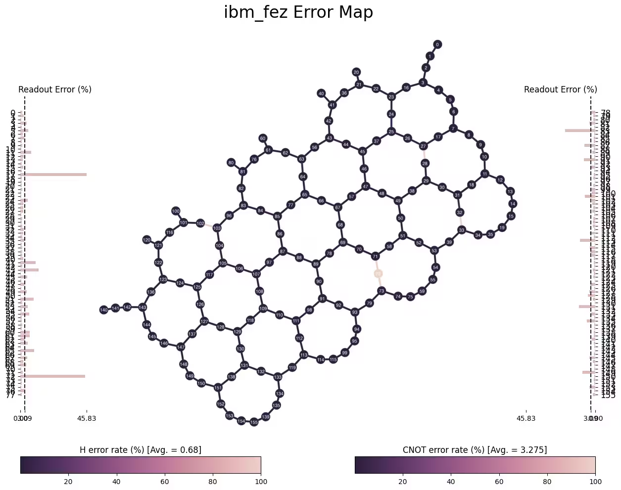
# Plot gate error map
# NOTE: These can change over time, so your results may look different
plot_error_map(backend)

bad_qubits = {
    56,
    63,
    67,
}  # qubits removed based on high coupling error (1.00)
good_qubits = list(set(range(backend.num_qubits)).difference(bad_qubits))
print("Physical qubits:\n", good_qubits)

Physical qubits:
 [0, 1, 2, 3, 4, 5, 6, 7, 8, 9, 10, 11, 12, 13, 14, 15, 16, 17, 18, 19, 20, 21, 22, 23, 24, 25, 26, 27, 28, 29, 30, 31, 32, 33, 34, 35, 36, 37, 38, 39, 40, 41, 42, 43, 44, 45, 46, 47, 48, 49, 50, 51, 52, 53, 54, 55, 57, 58, 59, 60, 61, 62, 64, 65, 66, 68, 69, 70, 71, 72, 73, 74, 75, 76, 77, 78, 79, 80, 81, 82, 83, 84, 85, 86, 87, 88, 89, 90, 91, 92, 93, 94, 95, 96, 97, 98, 99, 100, 101, 102, 103, 104, 105, 106, 107, 108, 109, 110, 111, 112, 113, 114, 115, 116, 117, 118, 119, 120, 121, 122, 123, 124, 125, 126, 127, 128, 129, 130, 131, 132, 133, 134, 135, 136, 137, 138, 139, 140, 141, 142, 143, 144, 145, 146, 147, 148, 149, 150, 151, 152, 153, 154, 155]

メインのトロッター回路生成

num_steps = 6
theta = Parameter("theta")
circuit = trotter_circuit(
    theta, layer_couplings, num_steps, qubits=good_qubits, backend=backend
)

後で割り当てるパラメータ値のリストを作成する

num_params = 12

# 12 parameter values for Rx between [0, pi/2].
# Reshape to outer product broadcast with observables
parameter_values = np.linspace(0, np.pi / 2, num_params).reshape(
    (num_params, 1)
)
num_params = parameter_values.size

ステップ 2: 量子ハードウェア実行のための問題の最適化

ISA 回路

回路をハードウェア上で実行する前に、ハードウェア実行向けに最適化する必要があります。このプロセスにはいくつかのステップが含まれます。

• 回路の仮想量子ビットをハードウェア上の物理量子ビットにマッピングする量子ビットレイアウトを選択します。
• 接続されていない量子ビット間の相互作用をルーティングするために、必要に応じてスワップゲートを挿入します。
• 回路内のゲートを、ハードウェア上で直接実行可能な命令セットアーキテクチャ（ISA）命令に変換します。
• 回路の深さとゲート数を最小化するための回路最適化を実行します。

Qiskit に組み込まれたトランスパイラはこれらのステップをすべて実行できますが、このチュートリアルでは、ユーティリティスケールの Trotter 回路をゼロから構築する方法を示します。適切な物理量子ビットを選択し、選択した量子ビットの接続されたペアにエンタングルメント層を定義します。ただし、回路内の非 ISA ゲートの変換や、トランスパイラが提供する回路最適化を利用する必要があります。

プリセットパスマネージャーを作成し、それを回路に対して実行することで、選択したバックエンド向けに回路をトランスパイルします。また、回路の初期レイアウトを、すでに選択済みの good_qubits に固定します。パスマネージャーを作成する簡単な方法は、generate_preset_pass_manager 関数を使用することです。パスマネージャーを使用したトランスパイルの詳細については、パスマネージャーによるトランスパイルを参照してください。

pm = generate_preset_pass_manager(
    backend=backend,
    initial_layout=good_qubits,
    layout_method="trivial",
    optimization_level=1,
)

isa_circuit = pm.run(circuit)

ISA オブザーバブル

次に、各仮想量子ビットに対して、必要な数の $\langle I \rangle$ 項をパディングして、すべての重み 1 の $\langle Z \rangle$ オブザーバブルを作成します。

observables = []
num_qubits = len(good_qubits)
for q in range(num_qubits):
    observables.append(
        SparsePauliOp("I" * (num_qubits - q - 1) + "Z" + "I" * q)
    )

トランスパイルプロセスにより、回路の仮想量子ビットがハードウェア上の物理量子ビットにマッピングされています。量子ビットレイアウトに関する情報は、トランスパイル済み回路の layout 属性に格納されています。オブザーバブルも仮想量子ビットの観点で定義されているため、このレイアウトをオブザーバブルに適用する必要があります。これは SparsePauliOp の apply_layout メソッドを使用して行います。

以下のコードブロックでは、各オブザーバブルがリストで囲まれていることに注目してください。これは、各量子ビットのオブザーバブルが各 theta 値に対して測定されるように、パラメータ値と_ブロードキャスト_するためです。プリミティブのブロードキャストルールはこちらで確認できます。

isa_observables = [
    [obs.apply_layout(layout=isa_circuit.layout)] for obs in observables
]

ステップ 3: Qiskit プリミティブを使用した実行

pub = (isa_circuit, isa_observables, parameter_values)

Estimator オプションの設定

次に、誤り軽減実験を実行するために必要な Estimator オプションを設定します。これには、エンタングルメント層のノイズ学習や ZNE 外挿のオプションが含まれます。

以下の設定を使用します。

# Experiment options
num_randomizations = 700
num_randomizations_learning = 40
max_batch_circuits = 3 * num_params
shots_per_randomization = 64
learning_pair_depths = [0, 1, 2, 4, 6, 12, 24]
noise_factors = [1, 1.3, 1.6]
extrapolated_noise_factors = np.linspace(0, max(noise_factors), 20)

# Base option formatting
options = {
    # Builtin resilience settings for ZNE
    "resilience": {
        "measure_mitigation": True,
        "zne_mitigation": True,
        # TREX noise learning configuration
        "measure_noise_learning": {
            "num_randomizations": num_randomizations_learning,
            "shots_per_randomization": 1024,
        },
        # PEA noise model configuration
        "layer_noise_learning": {
            "max_layers_to_learn": 3,
            "layer_pair_depths": learning_pair_depths,
            "shots_per_randomization": shots_per_randomization,
            "num_randomizations": num_randomizations_learning,
        },
        "zne": {
            "amplifier": "pea",
            "noise_factors": noise_factors,
            "extrapolator": ("exponential", "linear"),
            "extrapolated_noise_factors": extrapolated_noise_factors.tolist(),
        },
    },
    # Randomization configuration
    "twirling": {
        "num_randomizations": num_randomizations,
        "shots_per_randomization": shots_per_randomization,
        "strategy": "active-circuit",
    },
    # Optional Dynamical Decoupling (DD)
    "dynamical_decoupling": {"enable": True, "sequence_type": "XY4"},
}

ZNE オプションの説明

以下は、実験ブランチにおける追加オプションの詳細です。これらのオプションおよび名称は確定していないため、正式リリース前にすべて変更される可能性があることにご注意ください。

• amplifier: 意図したノイズファクターにノイズを増幅する際に使用する手法です。 許容される値は、2 量子ビット基底ゲートの繰り返しによって増幅する "gate_folding" と、 トワール済み 2 量子ビット基底ゲートの層に対する Pauli トワールノイズモデルを学習した後に 確率的サンプリングによって増幅する "pea" です。また、"gate_folding_front" および "gate_folding_back" オプションもあり、詳細は API ドキュメントで説明されています。
• extrapolated_noise_factors: 外挿モデルを評価するノイズファクター値を 1 つ以上指定します。値のシーケンスの場合、返される結果は、外挿モデルに対して指定されたノイズファクターが評価された配列値となります。値 0 はゼロノイズ外挿に対応します。

実験の実行

estimator = Estimator(mode=backend, options=options)
job = estimator.run([pub])

print(f"Job ID {job.job_id()}")

Job ID d0mcsvik4jhc73afljrg

ステップ 4: 後処理と古典形式での結果の返却

実験が完了したら、結果を確認できます。生の期待値と緩和された期待値を取得し、厳密な結果と比較します。次に、すべての量子ビットで平均化された各パラメータの期待値（緩和済み（外挿）と生）をプロットします。最後に、選択した個別の量子ビットの期待値をプロットします。

primitive_result = job.result()

一般的な結果の形状とメタデータ

PrimitiveResult オブジェクトには、PubResult というリスト状の構造が含まれています。Estimator に1つの PUB のみを送信するため、PrimitiveResult には単一の PubResult オブジェクトが含まれています。

PUB（primitive unified bloc）の結果の期待値と標準誤差は配列値です。ZNE を使用した Estimator ジョブの場合、PubResult の DataBin コンテナには期待値と標準誤差のいくつかのデータフィールドが利用可能です。ここでは期待値のデータフィールドについて簡単に説明します（標準誤差（stds）についても同様のデータフィールドが利用可能です）。

1. pub_result.data.evs: ゼロノイズに対応する期待値（ヒューリスティックに最良の外挿に基づく）。
   • 第1軸は、観測量 $\langle Z_i\rangle$ の仮想量子ビットインデックスです（$124$ 個の仮想量子ビット/観測量）
   • 第2軸は、$\theta$ のパラメータ値のインデックスです（$12$ 個のパラメータ値）
2. pub_result.data.evs_extrapolated: すべての外挿法に対する外挿されたノイズファクターの期待値。この配列には2つの追加軸があります。
   • 第3軸は外挿方法のインデックスです（$2$ 個の外挿法、exponential と linear）
   • 最後の軸は extrapolated_noise_factors のインデックスです（オプションで指定された $20$ 個の外挿ポイント）
3. pub_result.data.evs_noise_factors: 各ノイズファクターの生の期待値。
   • 第3軸は生の noise_factors のインデックスです（$3$ 個のファクター）

pub_result = primitive_result[0]

print(
    f"{pub_result.data.evs.shape=}\n"
    f"{pub_result.data.evs_extrapolated.shape=}\n"
    f"{pub_result.data.evs_noise_factors.shape=}\n"
)

pub_result.data.evs.shape=(153, 12)
pub_result.data.evs_extrapolated.shape=(153, 12, 2, 20)
pub_result.data.evs_noise_factors.shape=(153, 12, 3)

PrimitiveResult にはいくつかのメタデータフィールドも利用可能です。メタデータには以下が含まれます：

• resilience/zne/noise_factors: 生のノイズファクター
• resilience/zne/extrapolator: 各結果に使用された外挿法

primitive_result.metadata

{'dynamical_decoupling': {'enable': True,
  'sequence_type': 'XY4',
  'extra_slack_distribution': 'middle',
  'scheduling_method': 'alap'},
 'twirling': {'enable_gates': True,
  'enable_measure': True,
  'num_randomizations': 700,
  'shots_per_randomization': 64,
  'interleave_randomizations': True,
  'strategy': 'active-circuit'},
 'resilience': {'measure_mitigation': True,
  'zne_mitigation': True,
  'pec_mitigation': False,
  'zne': {'noise_factors': [1.0, 1.3, 1.6],
   'extrapolator': ['exponential', 'linear'],
   'extrapolated_noise_factors': [0.0,
    0.08421052631578947,
    0.16842105263157894,
    0.25263157894736843,
    0.3368421052631579,
    0.42105263157894735,
    0.5052631578947369,
    0.5894736842105263,
    0.6736842105263158,
    0.7578947368421053,
    0.8421052631578947,
    0.9263157894736842,
    1.0105263157894737,
    1.0947368421052632,
    1.1789473684210525,
    1.263157894736842,
    1.3473684210526315,
    1.431578947368421,
    1.5157894736842106,
    1.6]},
  'layer_noise_model': '<omitted for brevity>'}}

PubResult オブジェクトには、緩和に使用された学習済みノイズモデルに関する追加のレジリエンスメタデータがあります。

# Print learned layer noise metadata
for field, value in pub_result.metadata["resilience"]["layer_noise"].items():
    print(f"{field}: {value}")

noise_overhead: Infinity
total_mitigated_layers: 18
unique_mitigated_layers: 3
unique_mitigated_layers_noise_overhead: [1.4100369479435003e+44, 3.407263868699073e+112, 3.500660129782563e+37]

# Exact data computed using the methods described in the original reference
# Y. Kim et al. "Evidence for the utility of quantum computing before fault tolerance" (Nature 618, 500–505 (2023))
# Directly used here for brevity
exact_data = np.array(
    [
        1,
        0.9899,
        0.9531,
        0.8809,
        0.7536,
        0.5677,
        0.3545,
        0.1607,
        0.0539,
        0.0103,
        0.0012,
        0.0,
    ]
)

トロッターシミュレーション結果のプロット

以下のコードは、生の実験結果と緩和された実験結果を厳密解と比較するプロットを作成します。

"""Result visualization functions"""

def plot_trotter_results(
    pub_result: PubResult,
    angles: Sequence[float],
    plot_noise_factors: Sequence[float] | None = None,
    plot_extrapolator: Sequence[str] | None = None,
    exact: np.ndarray = None,
    close: bool = True,
):
    """Plot average magnetization from ZNE result data.
    Args:
        pub_result: The Estimator PubResult for the PEA experiment.
        angles: The Rx angle values for the experiment.
        plot_raw: If provided plot the unextrapolated data for the noise factors.
        plot_extrapolator: If provided plot all extrapolators, if False only plot
            the Automatic method.
        exact: Optional, the exact values to include in the plot. Should be a 1D
            array-like where the values represent exact magnetization.
        close: Close the Matplotlib figure before returning.
    Returns:
        The figure.
    """
    data = pub_result.data

    evs = data.evs
    num_qubits = evs.shape[0]
    num_params = evs.shape[1]
    angles = np.asarray(angles).ravel()
    if angles.shape != (num_params,):
        raise ValueError(
            f"Incorrect number of angles for input data {angles.size} != {num_params}"
        )

    # Take average magnetization of qubits and its standard error
    x_vals = angles / np.pi
    y_vals = np.mean(evs, axis=0)
    y_errs = np.std(evs, axis=0) / np.sqrt(num_qubits)

    fig, _ = plt.subplots(1, 1)

    # Plot auto method
    plt.errorbar(x_vals, y_vals, y_errs, fmt="o-", label="ZNE (automatic)")

    # Plot individual extrapolator results
    if plot_extrapolator:
        y_vals_extrap = np.mean(data.evs_extrapolated, axis=0)
        y_errs_extrap = np.std(data.evs_extrapolated, axis=0) / np.sqrt(
            num_qubits
        )
        for i, extrap in enumerate(plot_extrapolator):
            plt.errorbar(
                x_vals,
                y_vals_extrap[:, i, 0],
                y_errs_extrap[:, i, 0],
                fmt="s-.",
                alpha=0.5,
                label=f"ZNE ({extrap})",
            )

    # Plot raw results
    if plot_noise_factors:
        y_vals_raw = np.mean(data.evs_noise_factors, axis=0)
        y_errs_raw = np.std(data.evs_noise_factors, axis=0) / np.sqrt(
            num_qubits
        )
        for i, nf in enumerate(plot_noise_factors):
            plt.errorbar(
                x_vals,
                y_vals_raw[:, i],
                y_errs_raw[:, i],
                fmt="d:",
                alpha=0.5,
                label=f"Raw (nf={nf:.1f})",
            )

    # Plot exact data
    if exact is not None:
        plt.plot(x_vals, exact, "--", color="black", alpha=0.5, label="Exact")

    plt.ylim(-0.1, 1.2)
    plt.xlabel("θ/π")
    plt.ylabel(r"$\overline{\langle Z \rangle}$")
    plt.legend()
    plt.title(
        f"Error Mitigated Average Magnetization for Rx(θ) [{num_qubits}-qubit]"
    )
    if close:
        plt.close(fig)
    return fig

zne_metadata = primitive_result.metadata["resilience"]["zne"]
# Plot Trotter simulation results
fig = plot_trotter_results(
    pub_result,
    parameter_values,
    plot_extrapolator=zne_metadata["extrapolator"],
    plot_noise_factors=zne_metadata["noise_factors"],
    exact=exact_data,
)
display(fig)

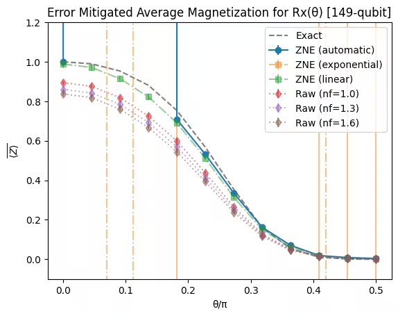
ノイズあり（ノイズファクター nf=1.0）の値は厳密値から大きく逸脱していますが、緩和された値は厳密値に近く、PEA ベースの緩和技術の有用性を示しています。

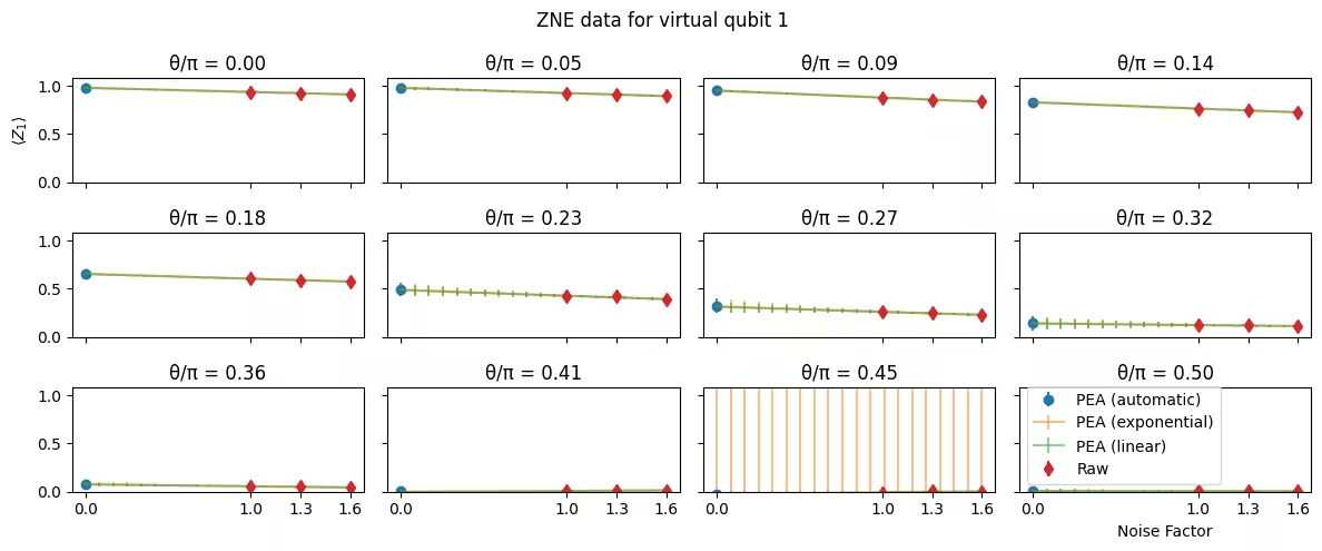
個別量子ビットの外挿結果のプロット

最後に、以下のコードは特定の量子ビットにおける異なるシータ値の外挿曲線を示すプロットを作成します。

def plot_qubit_zne_data(
    pub_result: PubResult,
    angles: Sequence[float],
    qubit: int,
    noise_factors: Sequence[float],
    extrapolator: Sequence[str] | None = None,
    extrapolated_noise_factors: Sequence[float] | None = None,
    num_cols: int | None = None,
    close: bool = True,
):
    """Plot ZNE extrapolation data for specific virtual qubit
    Args:
        pub_result: The Estimator PubResult for the PEA experiment.
        angles: The Rx theta angles used for the experiment.
        qubit: The virtual qubit index to plot.
        noise_factors: the raw noise factors.
        extrapolator: The extrapolator metadata for multiple extrapolators.
        extrapolated_noise_factors: The noise factors used for extrapolation.
        num_cols: The number of columns for the generated subplots.
        close: Close the Matplotlib figure before returning.
    Returns:
        The Matplotlib figure.
    """
    data = pub_result.data

    evs_auto = data.evs[qubit]
    stds_auto = data.stds[qubit]
    evs_extrap = data.evs_extrapolated[qubit]
    stds_extrap = data.stds_extrapolated[qubit]
    evs_raw = data.evs_noise_factors[qubit]
    stds_raw = data.stds_noise_factors[qubit]

    num_params = evs_auto.shape[0]
    angles = np.asarray(angles).ravel()
    if angles.shape != (num_params,):
        raise ValueError(
            f"Incorrect number of angles for input data {angles.size} != {num_params}"
        )

    # Make a square subplot
    num_cols = num_cols or int(np.ceil(np.sqrt(num_params)))
    num_rows = int(np.ceil(num_params / num_cols))
    fig, axes = plt.subplots(
        num_rows, num_cols, sharex=True, sharey=True, figsize=(12, 5)
    )
    fig.suptitle(f"ZNE data for virtual qubit {qubit}")

    for pidx, ax in zip(range(num_params), axes.flat):
        # Plot auto extrapolated
        ax.errorbar(
            0,
            evs_auto[pidx],
            stds_auto[pidx],
            fmt="o",
            label="PEA (automatic)",
        )

        # Plot extrapolators
        if (
            extrapolator is not None
            and extrapolated_noise_factors is not None
        ):
            for i, method in enumerate(extrapolator):
                ax.errorbar(
                    extrapolated_noise_factors,
                    evs_extrap[pidx, i],
                    stds_extrap[pidx, i],
                    fmt="-",
                    alpha=0.5,
                    label=f"PEA ({method})",
                )

        # Plot raw
        ax.errorbar(
            noise_factors, evs_raw[pidx], stds_raw[pidx], fmt="d", label="Raw"
        )

        ax.set_yticks([0, 0.5, 1, 1.5, 2])
        ax.set_ylim(0, max(1, 1.1 * max(evs_auto)))

        ax.set_xticks([0, *noise_factors])
        ax.set_title(f"θ/π = {angles[pidx]/np.pi:.2f}")
        if pidx == 0:
            ax.set_ylabel(r"$\langle Z_{" + str(qubit) + r"} \rangle$")
        if pidx == num_params - 1:
            ax.set_xlabel("Noise Factor")
            ax.legend()
    if close:
        plt.close(fig)
    return fig

virtual_qubit = 1
plot_qubit_zne_data(
    pub_result=pub_result,
    angles=parameter_values,
    qubit=virtual_qubit,
    noise_factors=zne_metadata["noise_factors"],
    extrapolator=zne_metadata["extrapolator"],
    extrapolated_noise_factors=zne_metadata["extrapolated_noise_factors"],
)

チュートリアルアンケート

このチュートリアルに関するフィードバックを提供するため、この短いアンケートにご協力ください。皆様のご意見は、コンテンツの提供とユーザーエクスペリエンスの改善に役立てさせていただきます。

アンケートへのリンク