VQEによるハイゼンベルグ鎖の基底状態エネルギー推定
使用量の目安: Heronプロセッサで約37分(注意: これはあくまで目安です。実際の実行時間は異なる場合があります。)
学習成果
このチュートリアルを完了すると、次の内容を理解できるようになります:
- QiskitでハイゼンベルグスピンチェーンをQuantum Hamiltonianとしてモデル化する方法
- SPSAオプティマイザーを使用して量子システムの基底状態エネルギーを推定する方法
- Qiskit RuntimeプリミティブとセッションによってIBM®量子ハードウェア上で変分ワークフローを実行する方法
前提知識
以下のトピックをあらかじめ学習しておくことをお勧めします:
背景
ハイゼンベルグスピンチェーンは、凝縮系物理学と量子磁性において最も広く研究されているモデルの一つです。最近接スピン間が交換相互作用によって結合している、相互作用する量子スピンの一次元格子を記述します。外部磁場を持つ等方性ハイゼンベルグモデルのハミルトニアンは次のように与えられます:
ここで、、はサイトに作用するパウリ演算子、総和は最近接ペアにわたって行われ、は交換結合定数(このチュートリアルでは等方的)、はサイト依存の外部磁場を表します。このチュートリアルでは、磁場の値はの区間からランダムにサンプリングされます。なお、以下の実装では「最近接」ペアの集合は、最初の個の量子ビット間のハードウェアバックエンドのネイティブ結合によって決定されるため、デバイスのトポロジーによっては厳密な直線鎖を形成しない場合があります。
このハミルトニアンの基底状態エネルギーを理解することは、物理学において根本的な重要性を持ちます。基底状態には、量子相転移・エンタングルメント構造・磁気秩序に関する情報が含まれています。古典的には、スピンの数が増えるにつれて正確な基底状態エネルギーの計算が困難になります。スピンのヒルベルト空間の次元はと指数的に増大するためです。これにより、量子シミュレーションの自然な候補となります。
変分量子固有値ソルバー(VQE)は、ハミルトニアンの基底状態エネルギーを推定するためのハイブリッド量子古典アルゴリズムです。量子コンピュータ上でパラメータ化された量子状態(アンザッツと呼ばれる)を準備し、期待値を測定することで機能します。その後、古典オプティマイザーがパラメータを反復的に調整してこのエネルギーを最小化します。測定されたエネルギーは常に真の基底状態エネルギーの上限であることを保証する変分原理を活用しています。
このチュートリアルでは、Qiskitの回路ライブラリからのefficient_su2アンザッツを使用します。これは一量子ビット回転とエンタングルゲートの層を構成します。最適化はSPSA(Simultaneous Perturbation Stochastic Approximation)アルゴリズムを使用して行われます。SPSAはパラメータ数に関わらず反復ごとにわずか2回の関数評価で勾配を推定するため、ノイズの多い量子ハードウェアに適しています。
前提条件
このチュートリアルを開始する前に、以下がインストールされていることを確認してください:
- Qiskit SDK v2.0以降(visualizationサポート付き)
- Qiskit Runtime v0.44以降(
pip install qiskit-ibm-runtime)
セットアップ
# Added by doQumentation — required packages for this notebook
!pip install -q matplotlib numpy qiskit qiskit-ibm-runtime
import numpy as np
import matplotlib.pyplot as plt
from typing import Sequence

from qiskit import QuantumCircuit
from qiskit.quantum_info import SparsePauliOp
from qiskit.primitives import BaseEstimatorV2
from qiskit.circuit.library import XGate
from qiskit.circuit.library import efficient_su2
from qiskit.transpiler import PassManager
from qiskit.transpiler.preset_passmanagers import generate_preset_pass_manager
from qiskit.transpiler.passes.scheduling import (
    ALAPScheduleAnalysis,
    PadDynamicalDecoupling,
)
from qiskit_ibm_runtime import QiskitRuntimeService, Session, EstimatorV2

def visualize_results(results):
    plt.plot(results["cost_history"], lw=2)
    plt.xlabel("Number of function evaluations")
    plt.ylabel("Energy")
    plt.show()
小規模な例
このセクションでは、ワークフローを構築しながら主要なコンポーネントを説明しつつ、Qiskitパターンの各ステップを小規模で実施します。
ステップ1: 古典的な入力を量子問題にマッピングする
- 入力: スピンの数
- 出力: ハイゼンベルグ鎖をモデル化するアンザッツとハミルトニアン
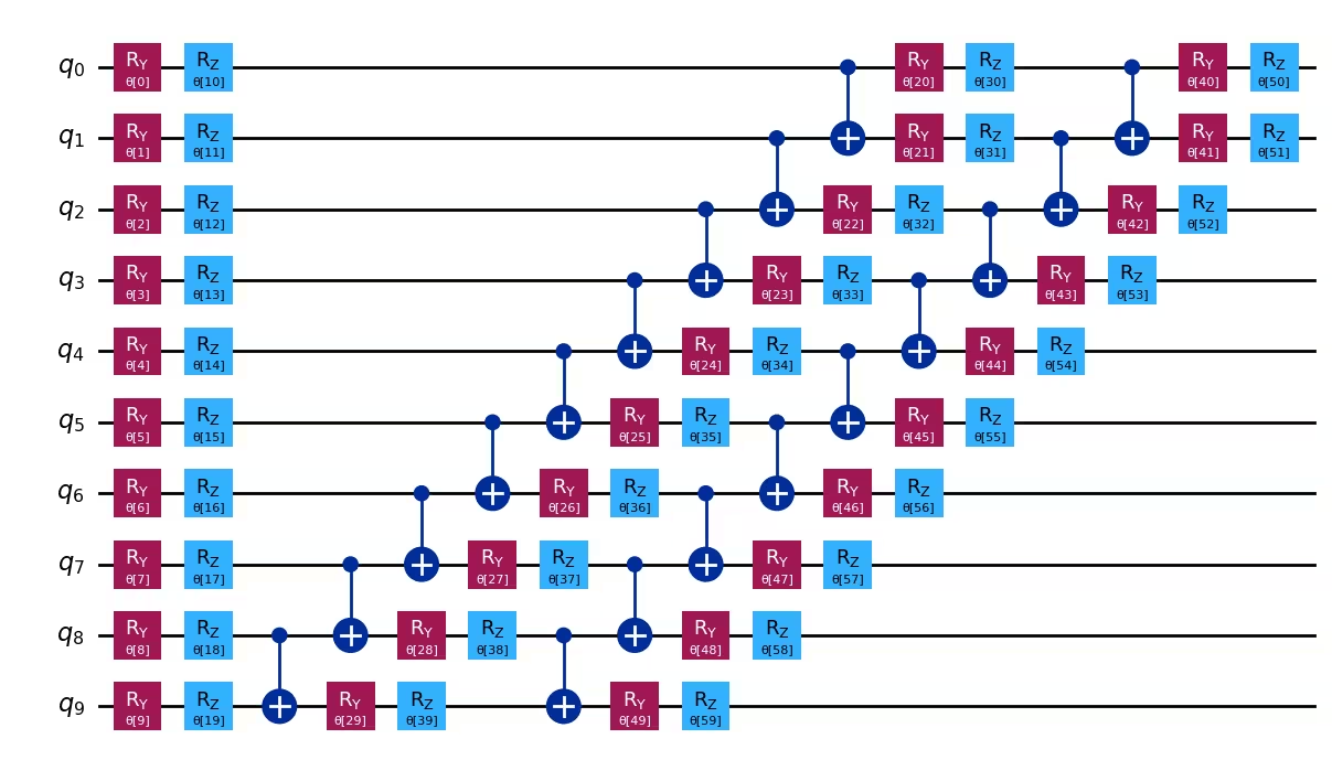
10スピンのハイゼンベルグ鎖をモデル化するアンザッツとハミルトニアンを構築します。このステップでは、最もビジーでないバックエンドの結合マップ上に10スピンのハイゼンベルグハミルトニアンを構築し、efficient_su2アンザッツを準備します。
num_spins = 10
ansatz = efficient_su2(num_qubits=num_spins, reps=2)

service = QiskitRuntimeService()
backend = service.least_busy(
    operational=True, min_num_qubits=num_spins, simulator=False
)

coupling = backend.target.build_coupling_map()
reduced_coupling = coupling.reduce(list(range(num_spins)))

edge_list = reduced_coupling.graph.edge_list()
ham_list = []

for edge in edge_list:
    ham_list.append(("ZZ", edge, 0.5))
    ham_list.append(("YY", edge, 0.5))
    ham_list.append(("XX", edge, 0.5))

for qubit in reduced_coupling.physical_qubits:
    ham_list.append(("Z", [qubit], np.random.random() * 2 - 1))

hamiltonian = SparsePauliOp.from_sparse_list(ham_list, num_qubits=num_spins)

ansatz.draw("mpl", style="iqp")
ステップ2: 量子ハードウェア実行向けに問題を最適化する
- 入力: 抽象回路、オブザーバブル
- 出力: 選択したQPU向けに最適化されたターゲット回路とオブザーバブル
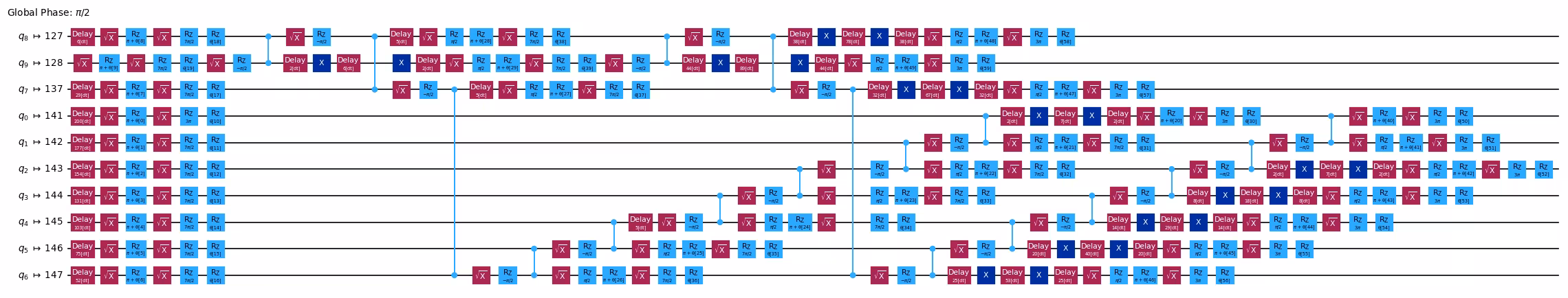
Qiskitのgenerate_preset_pass_manager関数を使用して、選択したQPUに対する回路の最適化ルーチンを自動的に生成します。プリセットパスマネージャーの中で最も高い最適化レベルを提供するoptimization_level=3を選択します。また、デコヒーレンスエラーを抑制するために、ALAPScheduleAnalysisおよびPadDynamicalDecouplingスケジューリングパスも組み込みます。
target = backend.target
pm = generate_preset_pass_manager(optimization_level=3, target=target)
pm.scheduling = PassManager(
    [
        ALAPScheduleAnalysis(durations=target.durations()),
        PadDynamicalDecoupling(
            durations=target.durations(),
            dd_sequence=[XGate(), XGate()],
            pulse_alignment=target.pulse_alignment,
        ),
    ]
)
isa_ansatz = pm.run(ansatz)
isa_observable = hamiltonian.apply_layout(isa_ansatz.layout)
isa_ansatz.draw("mpl", scale=0.6, style="iqp", fold=-1, idle_wires=False)
ステップ3: Qiskitプリミティブを使用して実行する
- 入力: ターゲット回路とオブザーバブル
- 出力: 最適化の結果
回路パラメータを最適化することで、システムの推定基底状態エネルギーを最小化します。最適化中のコスト関数の評価には、Qiskit RuntimeのEstimatorプリミティブを使用します。
ステップ2でバックエンド向けに回路を最適化したため、skip_transpilation=Trueを設定して最適化済みの回路を渡すことで、Runtimeサーバー上でのトランスパイルを省略できます。このデモでは、qiskit-ibm-runtimeプリミティブを使用してQPU上で実行します。qiskitの状態ベクトルベースのプリミティブで実行する場合は、Qiskit Runtimeプリミティブを使用しているコードブロックを、コメントアウトされたブロックに置き換えてください。
このチュートリアルでは、勾配ベースのオプティマイザーであるSPSA(Simultaneous Perturbation Stochastic Approximation)を使用します。次にその概要を説明し、Qiskit v2.0を使用してSPSAを実装するコードを提供します。
SPSAの紹介
SPSA(Simultaneous Perturbation Stochastic Approximation)[1]は、各反復において2回の関数呼び出しだけで勾配ベクトル全体を近似する最適化アルゴリズムです。を個のパラメータを最適化するコスト関数、を反復の番目のステップにおけるパラメータベクトルとします。勾配を計算するために、サイズのランダムベクトルが生成され、各要素( )はから一様にサンプリングされます。次に、ランダムベクトルの各要素に小さな値を掛けてランダム摂動を生成します。勾配は次のように推定されます。
直感的に、勾配推定時にランダム摂動が加えられるため、ノイズに起因するの厳密な値からの小さなずれは許容・吸収されると期待されます。実際、SPSAはノイズに対して特に頑健であることで知られており、各反復に必要なハードウェア呼び出しはわずか2回です。そのため、変分アルゴリズムの実装において非常に好まれるオプティマイザーの一つです。
このチュートリアルでは、番目の反復のハイパーパラメータおよびは次のように計算されます。
ここで定数値は、、、、です。これらの値は[2]から選択されています。SPSAから良好な性能を引き出すには、ハイパーパラメータの適切な調整が必要です。
def spsa(
    fun, x0, args=(), A=30, alpha=0.9, a=0.3, c=0.1, gamma=0.4, maxiter=100
):
    nparams = len(x0)
    x = np.copy(x0)

    for i in range(maxiter):
        a_i = a / (A + i + 1) ** alpha
        c_i = c / (i + 1) ** gamma
        delta_i = np.random.choice([-1, 1], nparams)

        # two hardware calls
        eval_1 = fun(x + c_i * delta_i, *args)
        eval_2 = fun(x - c_i * delta_i, *args)

        # compute the gradient and update the parameters
        grad = (eval_1 - eval_2) / (2 * c_i) * np.reciprocal(delta_i)
        x = x - a_i * grad

    return x
def cost_func(
    params: Sequence,
    ansatz: QuantumCircuit,
    hamiltonian: SparsePauliOp,
    estimator: BaseEstimatorV2,
    cost_history_dict: dict,
) -> float:
    """Ground state energy evaluation."""
    energy = (
        estimator.run([(ansatz, hamiltonian, [params])]).result()[0].data.evs
    )

    cost_history_dict["iters"] += 1
    cost_history_dict["prev_vector"] = list(params)
    cost_history_dict["cost_history"].append(float(energy[0]))

    print(
        f"Fx Iters. done: {cost_history_dict['iters']} [Current cost: {round(energy[0], 5)}]",
        end="\r",
    )

    return energy

def solve(x0, isa_ansatz, isa_observable, maxiter=150):
    cost_history_dict = {
        "prev_vector": None,
        "iters": 0,
        "cost_history": [],
        "y_min": None,
    }

    # Evaluate the problem using a QPU via Qiskit IBM Runtime
    with Session(backend=backend) as session:
        estimator = EstimatorV2(mode=session)
        estimator.skip_transpilation = True
        estimator.options.environment.job_tags = ["TUT_HSVQE"]
        x_opt = spsa(
            cost_func,
            x0=x0,
            args=(isa_ansatz, isa_observable, estimator, cost_history_dict),
            maxiter=maxiter,
        )

        y_min = cost_func(
            x_opt, isa_ansatz, isa_observable, estimator, cost_history_dict
        )

    return y_min, cost_history_dict
np.random.seed(42)
num_params = ansatz.num_parameters
params = 2 * np.pi * np.random.random(num_params)
ここではmaxiter = 50を設定します。各反復で勾配を計算するために2回の関数呼び出しが必要なため、関数呼び出しの総数はになります。より精度の高いエネルギー推定のためにmaxiterを任意の大きな値に増やすことができます。
maxiter = 50
spsa_min, spsa_history = solve(
    params, isa_ansatz, isa_observable, maxiter=maxiter
)
Fx Iters. done: 101 [Current cost: -3.03843]
ステップ4: 後処理を行い、結果を所望の古典的形式で返す
- 入力: 最適化中の基底状態エネルギー推定値
- 出力: 推定された基底状態エネルギー
print(f"Estimated ground state energy: {spsa_min}")
Estimated ground state energy: [-3.03842968]
results = {
    "spsa": spsa_history,
}

visualize_results(spsa_history)

大規模ハードウェアの例
このチュートリアルには大規模ハードウェアの例は含まれていません。量子ビット数が増えると、VQEはバレンプラトー現象によって大きな課題に直面します。コスト関数の勾配がシステムサイズとともに指数的に消失するため、大規模回路では最適化が実質的に不可能になります。ハードウェアノイズと組み合わさると、VQEを大きなスピンチェーンにスケールアップしても再現性のある結果を得ることができません。これらの制限を克服するアプローチについては、以下の「次のステップ」セクションをご参照ください。
チャレンジ
ハイゼンベルグ鎖のVQE実装が完成したら、次のことを試してみましょう:
- アンザッツの深さの実験:
efficient_su2のrepsパラメータを変更してください(例:reps=1やreps=3を試す)。アンザッツの深さは推定基底状態エネルギーと収束速度にどのような影響を与えますか?どの時点で収益逓減や不安定性が観察されますか? - SPSAハイパーパラメータの調整: 学習率スケジュールパラメータ(
a、c、alpha、gamma、A)を調整し、収束への影響を観察してください。ここで使用されているデフォルト値よりも速く収束する設定を見つけられますか? - 結合トポロジーの比較: バックエンドのネイティブ結合マップを使用する代わりに、単純な最近接直線チェーンを構築して結果を比較してください。物理ハードウェアの接続性は、トランスパイル後の回路深さと最終的なエネルギー推定にどのような影響を与えますか?
参考文献
[1] Spall, J. C. (2002). Implementation of the simultaneous perturbation algorithm for stochastic optimization. IEEE Transactions on Aerospace and Electronic Systems, 34(3), 817-823.
[2] Sahin, M. Emre, et al. (2025). Qiskit Machine Learning: an open-source library for quantum machine learning tasks at scale on quantum hardware and classical simulators. arXiv:2505.17756.
次のステップ
この内容が興味深いと感じた方は、以下の資料もご覧ください:
- サンプルベース量子対角化(SQD)を試す: このチュートリアルで示されているように、VQEはバレンプラトーと高い測定オーバーヘッドにより大規模では大きな課題に直面します。IBMは、よりスケーラブルな代替手段としてサンプルベース量子対角化(SQD)を開発しました。VQEとは異なり、SQDは変分最適化を完全に回避します。量子コンピュータがサンプルを生成し、古典コンピュータがそれらのサンプルによってスパンされる部分空間にハミルトニアンを射影して対角化します。これにより、バレンプラトーの影響を受けることなく、大幅に少ない測定回数で基底状態エネルギーの上限が得られます。SQDチュートリアルに従って、このアプローチを実際に確認してください。
- 量子対角化アルゴリズムコースの探索: IBM Quantum Learningの量子対角化アルゴリズムコースで、VQEとSQDの両方のトレードオフを含む理解を深めてください。