Greenberger-Horne-Zeilinger状態のシャドウトモグラフィー

使用量の目安: Heron r2プロセッサーで10秒未満(注: これはあくまで目安です。実際の実行時間は異なる場合があります。)

学習内容

• シャドウトモグラフィーが量子状態の古典シャドウをどのように構築するか、そしてなぜ完全な状態トモグラフィーよりも指数関数的に少ない測定回数で済むのか

• Qiskitを使って局所パウリシャドウトモグラフィーを実装し、単一量子ビットの磁化、2点相関関数、2量子ビット縮約密度行列を推定する方法

• 大規模なハードウェア実験で、時空間コードを用いた低オーバーヘッドのエラー検出のために qiskit-paulice を使用する方法

前提知識

• 測定

• 量子状態トモグラフィー

• 時空間コードを用いたエラー検出

背景

$N$ 量子ビット系の完全な量子状態トモグラフィーでは、密度行列の独立なパラメーター $4^N -1$ 個すべてを推定するために、指数関数的に多くの測定が必要です。たとえば50量子ビットの系では、このプロセスにおよそ $10^{30}$ ショットが必要で、これは観測可能な宇宙の星の数の10億倍以上です。シャドウトモグラフィー [1] は、量子状態の「古典シャドウ」を構築する量子情報プロトコルです。古典シャドウからは、observable の数に対して対数的にしか増えず、系のサイズ $N$ に依存しないショット数で目的の observable を推定できます。このため、エネルギー推定、エンタングルメントエントロピーや相関関数の計算、量子機械学習におけるカーネル推定など、量子コンピューティングの多くの分野で重要です。

このチュートリアルでは、シャドウトモグラフィーを使って、強くエンタングルしたGreenberger-Horne-Zeilinger(GHZ)状態の局所 observable、すなわち量子ビット $i$ の単一量子ビット磁化 $\langle Z_i \rangle$、2点相関関数 $\langle Z_i Z_j\rangle$、2量子ビット縮約密度行列(2-RDM)を推定する方法を示します。まず、ステートベクターシミュレーションを使って10量子ビットのGHZ状態に対する小規模なシャドウトモグラフィーのワークフローを説明し、続いて実際の量子ハードウェア上での100量子ビットのデモンストレーションを示します。

シャドウトモグラフィーのプロトコル

シャドウトモグラフィーのプロトコルは次のステップで構成されます。

1. ユニタリーのアンサンブルから抽出したランダムなユニタリー $U$ を初期の量子状態に適用します。
2. 計算基底で結果を測定し、ビット列 $\ket{b}$ を得ます。
3. 古典スナップショット $\hat{\rho} = \mathcal{M}^{-1}(U^{\dagger}\ket{b}\bra{b}U)$ を保存します。ここで $\mathcal{M}^{-1}$ は測定チャネル $\mathcal{M}(\rho)=\mathbb{E}[U^{\dagger}\ket{b}\bra{b}U]$ の逆です。
4. このプロセスを $T$ 回繰り返します。$T$ 個のスナップショットの集合 $\{\hat{\rho}_t\}$ が古典シャドウ $S(\rho, T)$ を形成します。
5. 演算子 $O$ の observable $o$ を $\frac{1}{T}\sum_{t=1}^{T}\text{Tr}(O\hat{\rho}_t)$ として推定します。

シャドウトモグラフィーの種類

プロトコルのステップ1におけるユニタリーアンサンブル(つまり基底)の選択は、与えられたシャドウトモグラフィーのサンプル複雑度、推定値の分散、情報の完全性に影響します。文献では多くのアンサンブル群が検討されており、それぞれに複雑さと observable の推定効率のトレードオフがあります。最もよく使われる種類の特性を次の表にまとめます。ただし、このリストがすべてではありません。

種類	アンサンブル	サンプル複雑度	回路深さ	適した observable
局所パウリ [1]	単一量子ビットのパウリ演算子 $\{X, Y, Z\}$	$\mathcal{O}(3^k\text{log}M/\varepsilon^2)$	1	局所/少数体
グローバルClifford [1]	$N$ 量子ビットのClifford	$\mathcal{O}(\text{Tr}(O^2)\text{log}M/\varepsilon^2)$	$\mathcal{O}(N\text{log}N)$	低ランク、フィデリティ
フェルミオンガウシアン [2], [3]	マッチゲート回路	$\mathcal{O}(\binom{\mu}{k}\frac{1}{\varepsilon^2})$	$\mathcal{O}(N^2)$	フェルミオン
浅いシャドウ [4], [5]	低深さ回路	$\mathcal{O}(k2^k\text{log}M/\varepsilon^2)$	$\mathcal{O}(\text{log}N)$	非局所(ハードウェアに適している)

表で使われている用語の定義は次のとおりです。

• 「サンプル複雑度」は、特定のシャドウトモグラフィーの種類に必要な測定回数を指します。

• 「回路深さ」は、量子ハードウェア上で測定を実装するコストの大きさを表します。

• $N$ は量子ビット数です。

• $k$ は observable の局所性です(たとえば、$\langle Z_i \rangle$ は $k=1$、$\langle Z_i Z_j\rangle$ は $k=2$ です)。

• $M$ は同時に推定する observable の数です。

• $\varepsilon$ は加法誤差の許容値です。

• $\mu$ はフェルミオンの数です。

局所パウリアンサンブルは最もハードウェアに適していますが、$3^k$ のサンプル複雑度のペナルティがあるため、非局所的な性質の推定には不向きです。より一般的には、局所シャドウのサンプル複雑度の上界は $4^k$ でスケールし、テンソル積 observable という特殊な場合には $3^k$ に改善されます。

逆に、グローバルCliffordアンサンブルは非局所 observable の推定に使えますが、回路深さの点で不利です。フェルミオンガウシアンシャドウは、多体物理、化学、材料のシミュレーションで有用ですが、マッチゲート回路を必要とし、汎用のゲート型デバイスでは大きなオーバーヘッドを伴う可能性があります。

浅いシャドウは、局所パウリとグローバルCliffordの中間の回路深さを持つため、実用的な実装に非常に有望な種類です。ただし、特定の observable に対する最適な回路深さについては、まだ未解決の問題がいくつか残っています。

シャドウトモグラフィーの研究が最前線で拡大し続ける中、取り組むべき最も関連性の高い問題には、対象の observable の集合に対する測定アンサンブルの最適な選択、サンプル複雑度の上界の改善、時間発展した observable へのプロトコルの拡張などがあります。それでもシャドウトモグラフィーは、最小限の測定回数で量子状態から最大限の古典情報を引き出す主要なワークフローの1つであり、完全なトモグラフィーも古典シミュレーションも不可能な規模での量子状態の特性評価に最適です。

局所パウリアンサンブル

このチュートリアルでは、ランダムなパウリ基底、すなわち単一量子ビットのClifford ゲートを使ってシャドウを収集し、GHZ状態の性質を推定します。パウリ測定は局所 observable(スピン密度、局所相関関数、位置確率密度など)の推定には優れた選択ですが、グローバルな observable(全エネルギー、運動量、電荷など)には適していません。

ここでは、量子ビットごとにランダムなパウリ基底 $\{X, Y, Z\}$ を独立に選び、対応する単一量子ビット回転を適用してから測定します。

$$\begin{equation} U = U_0 \otimes U_1 \otimes \cdots \otimes U_{n-1}, U_q \in \{I, H, S^{\dagger}H\} \end{equation} \tag{1}$$

このアンサンブルでは、測定チャネルの逆は次のとおりです。

$$\begin{equation} \hat{\rho}_q=3U_q^{\dagger}\ket{b_q}\bra{b_q}U_q - I \end{equation} \tag{2}$$

係数 $3$ は3つのパウリ基底の平均から生じ、パラメーター $\frac{1}{3}$ の脱分極チャネルを生み出します。完全な推定量は、単一量子ビット推定量の積に分解されます。表に示したように、局所性 $k$ の $M$ 個の observable について、すべての observable を加法誤差 $\varepsilon$ まで高い確率で推定するのに必要なパウリシャドウの数は $\mathcal{O}(\frac{3^k\text{log}(M)}{\varepsilon^2})$ です。observable が局所的である限り、系のサイズは測定コストに影響しないため、指数関数的に多くの observable を対数的なコストだけで同時に推定できます。

平均値の中央値

$T$ 個のスナップショットの単純平均は、observable の単一ショット推定の分散を $\frac{1}{T}$ のように減らしますが、外れ値の影響を受けやすいという欠点があります。これを改善するために、平均値の中央値(median of means)を使用できます。手順は次のとおりです。

• $T$ 個のスナップショットを $K$ 個の同じサイズのグループに分割する
• 各グループ内で平均を計算する
• グループ平均の中央値を返す

このチュートリアルでは、局所パウリシャドウトモグラフィーを実行してGHZ状態の性質を推定します。まず10量子ビットのシミュレーション例を用い、その後100量子ビットのハードウェア実験を示します。

要件

このチュートリアルを始める前に、次のものがインストールされていることを確認してください。

• 可視化サポート付きのQiskit SDK v2.0以降

• IBM Quantum Compute v0.28以降(pip install qiskit-ibm-runtime)

• Qiskit Paulice(pip install qiskit-paulice)

セットアップ

# Added by doQumentation — installs the packages this notebook needs if they are missing
import importlib.util

_needed = {"matplotlib": "matplotlib", "numpy": "numpy", "qiskit": "qiskit", "qiskit_ibm_runtime": "qiskit-ibm-runtime", "qiskit_paulice": "qiskit-paulice"}
_missing = [pip for module, pip in _needed.items()
            if importlib.util.find_spec(module) is None]
# One at a time, so a package that fails to install does not block the others
for _pip in _missing:
    %pip install -q {_pip}
if not _missing:
    print("\u2713 All required packages are installed")

import numpy as np
import matplotlib.pyplot as plt
from collections import deque, defaultdict
from qiskit import QuantumCircuit, ClassicalRegister
from qiskit.quantum_info import (
    Statevector,
    partial_trace,
    Operator,
    Pauli,
    SparsePauliOp,
)
from qiskit.transpiler import generate_preset_pass_manager
from qiskit_ibm_runtime import QiskitRuntimeService
from qiskit_ibm_runtime import SamplerV2 as Sampler
from qiskit_paulice.layout import get_low_overhead_ancillas

seed = 42  # for reproducibility
rng = np.random.default_rng(seed)

チュートリアルの後半の大規模ハードウェアの例では、次のヘルパー関数を使用します。

• bad_cz、bad_readout、bad_coherence — バックエンドのキャリブレーションデータを照会し、エラーやコヒーレンスのしきい値を超えているゲート、量子ビット、エッジを特定して、回路レイアウトから除外できるようにします。

• parallel_ghz — カップリングマップに対する幅優先探索を使って、指定したサイズのGHZ回路を構築し、CNOT層を並列に配置して回路深さを最小化します。

• weighted_coverage、active_wires、z_trace_backward — [6] の逆伝播手法を使って、指定した時空間パリティチェックの集合により、GHZ回路のエラー面のどれだけが保護されるかを計算します。

• add_measurements — GHZ量子ビットとチェック量子ビットの測定を別々の古典レジスターに追加し、独立に事後選択できるようにします。

• build_shadow_circuits — 測定の前に適切な単一量子ビット回転を追加して、ランダムなパウリ基底ごとに1つの回路を生成します。

• parse_hw_results_w_checks — Samplerの出力を、ショットごとに1つの (ghz_bits, check_bits, bases) の三つ組に展開します。

• adapt_to_flat_bits、estimate_zz_nn_hw — GHZレジスターのビットをデバイス全体のインデックス空間にマッピングし直し、中央値の平均による $\langle Z_i Z_{i+1}\rangle$ の推定値を計算します。

def bad_cz(target, threshold: float = 0.01) -> list:
    "Return edges whose CZ error exceeds threshold."
    edges = []
    for edge in backend.target.build_coupling_map().get_edges():
        if (edge[1], edge[0]) not in edges:
            edges.append(edge)
    cz_errors = {edge: target["cz"][edge].error for edge in edges}
    worst = sorted(cz_errors.items(), key=lambda x: x[1], reverse=True)
    return [list(edge) for edge, error in worst if error > threshold]

def bad_readout(target, threshold: float = 0.01) -> list:
    "Return nodes whose measurement error exceeds threshold."
    meas_errors = {
        node: target["measure"][(node,)].error
        for node in range(backend.num_qubits)
    }
    worst = sorted(meas_errors.items(), key=lambda x: x[1], reverse=True)
    return [node for node, error in worst if error > threshold]

def bad_coherence(target, threshold: float = 60) -> list:
    "Return nodes whose T2 value is below threshold."
    t2s = {
        node: (target.qubit_properties[node].t2 or 0) * 1e6
        for node in range(backend.num_qubits)
    }
    return [
        node
        for node, val in sorted(t2s.items(), key=lambda x: x[1])
        if val < threshold
    ]

def parallel_ghz(
    root: int, num_qubits: int, backend, bad_edges: list, skip: list
) -> tuple:
    "Build a GHZ circuit of size num_qubits using BFS from root, one neighbor per layer."
    edges = [
        e
        for e in [list(e) for e in backend.coupling_map.get_edges()]
        if e not in bad_edges
        and [e[1], e[0]] not in bad_edges
        and e[0] not in skip
        and e[1] not in skip
    ]
    adj = defaultdict(list)
    for u, v in edges:
        adj[u].append(v)
        adj[v].append(u)

    qc = QuantumCircuit(backend.num_qubits)
    visited = [root]
    queue = deque([root])
    explored = defaultdict(set)
    layers = []
    qc.h(root)

    while queue and len(visited) < num_qubits:
        layer = []
        for node in list(queue):
            queue.popleft()
            unvisited = [
                nb
                for nb in adj[node]
                if nb not in visited and nb not in explored[node]
            ]
            if unvisited:
                nb = unvisited[0]
                visited.append(nb)
                queue.append(node)
                queue.append(nb)
                explored[node].add(nb)
                layer.append((node, nb))
                if len(visited) == num_qubits:
                    break
        if layer:
            layers.append(layer)
        else:
            break

    for layer in layers:
        for q1, q2 in layer:
            qc.cx(q1, q2)
        qc.barrier()

    return qc, visited, layers

def weighted_coverage(
    layers: list, parities: list, w_idle: float = 0.2, w_gate: float = 0.8
) -> float:
    "Compute weighted fraction of wires covered by at least one parity check."
    wires = active_wires(layers)
    covered_by_any = {n_layer: set() for n_layer in range(len(layers))}
    for parity in parities:
        for n_layer, qs in z_trace_backward(layers, parity).items():
            covered_by_any[n_layer] |= qs
    covered_weight = total_weight = 0
    for n_layer in range(len(layers)):
        idle = wires[n_layer]["idle"]
        gate = wires[n_layer]["gate"]
        total_weight += w_idle * len(idle) + w_gate * len(gate)
        covered_weight += w_idle * len(
            covered_by_any[n_layer] & idle
        ) + w_gate * len(covered_by_any[n_layer] & gate)
    return covered_weight / total_weight if total_weight > 0 else 0

def active_wires(layers: list) -> dict:
    """
    Returns per-layer dict with two sets:
    - 'idle': activated wires that are idle in this layer
    - 'gate': activated wires that are control/target of a CNOT at this layer
    """
    first_activation = {}
    for n_layer, layer in enumerate(layers):
        for c, t in layer:
            first_activation.setdefault(c, n_layer)
            first_activation.setdefault(t, n_layer)
    result = {}
    for n_layer in range(len(layers)):
        active = {
            q
            for q, n_layer0 in first_activation.items()
            if n_layer >= n_layer0
        }
        gate = {q for c, t in layers[n_layer] for q in (c, t)}
        result[n_layer] = {"idle": active - gate, "gate": gate}
    return result

def z_trace_backward(layers: list, initial_Zs: list) -> dict:
    """
    Backward propagate Zs with parity cancellation.
    Returns {layer: set of qubits with odd parity Z at that layer}.
    """
    wires = active_wires(layers)
    support = set(initial_Zs)
    trace = {}
    for n_layer in range(len(layers) - 1, -1, -1):
        active = wires[n_layer]["idle"] | wires[n_layer]["gate"]
        trace[n_layer] = support & active
        new_support = set()
        for q in support:
            hit = False
            for c, t in layers[n_layer]:
                if q == t:
                    new_support ^= {t, c}
                    hit = True
                    break
                elif q == c:
                    new_support ^= {c}
                    hit = True
                    break
            if not hit:
                new_support ^= {q}
        support = new_support
    return trace

def add_measurements(
    qc: QuantumCircuit, ghz_qubits: list, checks: list
) -> QuantumCircuit:
    "Add GHZ and check qubit measurements into separate classical registers."
    c1 = ClassicalRegister(len(ghz_qubits), "c1")
    qc.add_register(c1)
    for q, c in zip(ghz_qubits, c1):
        qc.measure(q, c)
    c2 = ClassicalRegister(len(checks), "c2")
    qc.add_register(c2)
    for q, c in zip(checks, c2):
        qc.measure(q, c)
    return qc

def build_shadow_circuits(
    base_circuit: QuantumCircuit,
    n_measure: int,
    ghz_qubits: list,
    checks: list,
) -> tuple:
    "Build n_measure circuits by appending random Pauli basis rotations to each GHZ qubit."
    n = base_circuit.num_qubits
    all_bases = rng.integers(0, 3, size=(n_measure, n))
    circuits = []
    for m in range(n_measure):
        qc = base_circuit.copy()
        qc.barrier()
        for q in ghz_qubits:
            b = all_bases[m, q]
            if b == 1:
                qc.h(q)
            elif b == 2:
                qc.sdg(q)
                qc.h(q)
        add_measurements(qc, ghz_qubits, checks)
        circuits.append(qc)
    return circuits, all_bases

def parse_hw_results_w_checks(
    result, bases: np.ndarray, ghz_qubits: list, checks: list
) -> list:
    "Parse hardware bitstrings into (ghz_bits, check_bits, bases) triples."
    snapshots = []
    n_ghz = len(ghz_qubits)
    n_checks = len(checks)
    for t, pub_result in enumerate(result):
        ghz_strings = (
            pub_result.data.c1.get_bitstrings()
        )  # one entry per shot
        chk_strings = pub_result.data.c2.get_bitstrings()
        for ghz_bitstring, check_bitstring in zip(ghz_strings, chk_strings):
            ghz_bits = [
                int(ghz_bitstring[n_ghz - 1 - i]) for i in range(n_ghz)
            ]
            check_bits = [
                int(check_bitstring[n_checks - 1 - i])
                for i in range(n_checks)
            ]
            snapshots.append((ghz_bits, check_bits, bases[t]))
    return snapshots

def adapt_to_flat_bits(
    ghz_bits: list, ghz_qubits: list, n_total: int
) -> list:
    "Map GHZ-register bits back to a full n_total-length bit vector."
    bits = [0] * n_total
    for i, q in enumerate(ghz_qubits):
        bits[q] = ghz_bits[i]
    return bits

def estimate_zz_nn_hw(
    snapshots: list, ghz_qubits: list, n_total: int, n_groups: int
) -> np.ndarray:
    "Estimate <ZiZi+1> for each neighboring GHZ qubit pair from flat-bit snapshots."
    pairs = list(zip(ghz_qubits[:-1], ghz_qubits[1:]))
    all_est = np.column_stack(
        [
            snapshot_estimate(
                ["Z" if q in pair else "I" for q in range(n_total)], snapshots
            )
            for pair in pairs
        ]
    )
    return mom(all_est, n_groups).real

小規模シミュレーターの例

まず、ステートベクターシミュレーションを使って10量子ビットのGHZ状態を準備し、局所パウリシャドウを使ってその性質を推定します。GHZ状態は3量子ビット以上の最大エンタングル状態で、多体エンタングルメントのベンチマークとして使われます。量子通信や暗号プロトコルの一般的な構成要素でもあります。さらに、GHZ回路の解析的な性質は完全にわかっているため、このチュートリアルでの検証に最適です。

ステップ1: 古典入力を量子問題にマッピングする

理想的な10量子ビットのGHZ状態を準備します。

def ghz_statevector(num_qubits):
    qc = QuantumCircuit(num_qubits)
    qc.h(0)
    for q in range(num_qubits - 1):
        qc.cx(q, q + 1)
    return Statevector(qc)

num_qubits = 10  # number of qubits
psi = ghz_statevector(num_qubits)
psi.seed(seed)
print(
    f"{num_qubits}-qubit GHZ state ready (norm = {np.linalg.norm(psi):.6f})"
)

10-qubit GHZ state ready (norm = 1.000000)

ステップ2: 量子ハードウェアでの実行に向けて最適化する

次に、GHZ状態をランダムなパウリ基底に回転させてシャドウスナップショットを収集する関数を定義します。これは、大規模な例でSamplerプリミティブがハードウェア上で行うことを再現したものです。

def basis_circuit(b):
    """0 -> Z basis (I), 1 -> X basis (H), 2 -> Y basis (Sdg;H)."""
    qc = QuantumCircuit(1)
    if b == 1:
        qc.h(0)
    elif b == 2:
        qc.sdg(0)
        qc.h(0)
    # b == 0: Z basis, no rotation
    return qc

_basis = {
    b: basis_circuit(b) for b in (0, 1, 2)
}  # built once, shared with the estimator's _U

def collect_shadow_snapshots(psi, n_snapshots, num_qubits):
    snapshots = []
    for _ in range(n_snapshots):
        bases = rng.integers(0, 3, size=num_qubits)
        rot = QuantumCircuit(num_qubits)
        for q, b in enumerate(bases):
            rot.compose(_basis[b], qubits=[q], inplace=True)
        evolved = psi.evolve(rot)
        evolved.seed(int(rng.integers(0, 2**31)))
        bitstr = next(
            iter(evolved.sample_counts(shots=1))
        )  # Born rule internal
        bits = [int(x) for x in bitstr[::-1]]  # little-endian -> qubit
        snapshots.append((bits, bases))
    return snapshots

ステップ3: Qiskitプリミティブを使って実行する

このシミュレーションでは、ステートベクターを直接使用します。

n_snapshots = 5000  # number of shadow snapshots
n_groups = 20  # groups/batches for median-of-means

snapshots = collect_shadow_snapshots(psi, n_snapshots, num_qubits)
print(f"Collected {n_snapshots} snapshots.")

Collected 5000 snapshots.

ステップ4: 後処理を行い、目的の古典形式で結果を返す

シャドウ・スナップショットの収集に使用するランダムな測定基底に対して、シャドウ推定量とメディアン・オブ・ミーンズ（MOM）推定量を定義します。これらの関数を使用して、収集した測定結果からGHZ状態の特性（単一量子ビットの磁化、2量子ビット相関子、2量子ビットRDMなど）を推定します。その後、推定値を厳密値と比較します。

_U = {
    b: Operator(basis_circuit(b)) for b in (0, 1, 2)
}  # rotation Uᵢ per basis
_P = {p: Operator(Pauli(p)) for p in "IXYZ"}  # single-qubit Paulis

def shadow_estimator(P, b, bit):  # P is a label char, e.g. "X"
    UPU = _U[b] @ _P[P] @ _U[b].adjoint()  # Uᵢ P Uᵢ†
    return (3 * UPU.data[bit, bit] - np.trace(_P[P].data)).real

def mom(estimates: np.ndarray, n_groups: int) -> np.ndarray:
    "Median-of-means outlier suppression."
    T = len(estimates)
    spg = T // n_groups  # shots per group
    trimmed = estimates[
        : spg * n_groups
    ]  # drop any leftover shots that don't cleanly fit into a group
    groups = trimmed.reshape(n_groups, spg, *estimates.shape[1:])
    means = groups.mean(axis=1)  # take the mean of each group
    return np.median(means.real, axis=0) + 1j * np.median(
        means.imag, axis=0
    )  # take the median of means for real and imaginary parts separately

def snapshot_estimate(
    pauli_string, snapshots
):  # full-width label, len == num_qubits
    out = np.empty(len(snapshots), dtype=complex)
    for t, (bits, bases) in enumerate(snapshots):
        e = 1.0 + 0j
        for q, P in enumerate(pauli_string):
            e *= shadow_estimator(P, bases[q], bits[q])
        out[t] = e
    return out

Z_est = np.column_stack(
    [
        snapshot_estimate(
            ["Z" if q == i else "I" for q in range(num_qubits)], snapshots
        )
        for i in range(num_qubits)
    ]
)
Z_vals = mom(Z_est, n_groups).real

ZZ_est = np.column_stack(
    [
        snapshot_estimate(
            ["Z" if q in (i, i + 1) else "I" for q in range(num_qubits)],
            snapshots,
        )
        for i in range(num_qubits - 1)
    ]
)
ZZ_nn = mom(ZZ_est, n_groups).real

ZZ_full = np.zeros((n_snapshots, num_qubits, num_qubits), dtype=complex)
for i in range(num_qubits):
    ZZ_full[:, i, i] = 1.0  # diagonal is always 1
    for j in range(i + 1, num_qubits):
        col = snapshot_estimate(
            ["Z" if q in (i, j) else "I" for q in range(num_qubits)],
            snapshots,
        )
        ZZ_full[:, i, j] = col
        ZZ_full[:, j, i] = col  # symmetric
ZZ_mat = mom(ZZ_full, n_groups).real

# 2-qubit reduced density matrix (RDM) for pair (qi, qj)
# the elementwise complex median (real/imag split) for the RDM coefficients generalizes the scalar median in Ref.[1]
qi, qj = 0, num_qubits - 1
terms = []
for a in "IXYZ":
    for b in "IXYZ":
        label = "".join({qi: a, qj: b}.get(q, "I") for q in range(num_qubits))
        c = mom(snapshot_estimate(label, snapshots).reshape(-1, 1), n_groups)[
            0
        ]
        terms.append((b + a, c / 4))
rho_shadow = SparsePauliOp.from_list(terms).to_matrix()

traced_out = [q for q in range(num_qubits) if q not in (qi, qj)]
rho_exact = partial_trace(
    psi, traced_out
).data  # diag(0.5, 0, 0, 0.5) for GHZ

print(f"{'Observable':<22} {'Estimated':>12} {'Ideal':>8} {'Max error':>12}")
print("-" * 57)
print(
    f"{'<Zi> (all qubits)':<22} {'-':>12} {'0':>8} {np.max(np.abs(Z_vals)):>12.4f}"
)
print(
    f"{'<ZiZi+1> mean':<22} {np.mean(ZZ_nn):>12.4f} {'1':>8} {np.max(np.abs(ZZ_nn - 1)):>12.4f}"
)
print(
    f"{'2-RDM Frobenius err':<22} {'-':>12} {'0':>8} {np.linalg.norm(rho_shadow - rho_exact):>12.4f}"
)

Observable                Estimated    Ideal    Max error
---------------------------------------------------------
<Zi> (all qubits)                 -        0       0.0540
<ZiZi+1> mean                1.0040        1       0.1520
2-RDM Frobenius err               -        0       0.1080

結果の可視化

最初のプロットは、各量子ビットについて推定された単一量子ビットの磁化の値を示しています。2番目のプロットは、すべての量子ビット・ペアについて推定された2点相関子の値の分布を示しています。最後のプロットは、2量子ビット縮約密度行列の成分の大きさを示しています。与えられた系のサイズに対して、かなり多くのスナップショットを使用しているため、結果は厳密な値に近くなっています。

fig, axes = plt.subplots(
    1, 3, figsize=(14, 4), gridspec_kw={"width_ratios": [1, 1, 1]}
)

z_exact = psi.expectation_value(
    SparsePauliOp.from_sparse_list([("Z", [0], 1.0)], num_qubits)
).real  # 0.0
zz_exact = psi.expectation_value(
    SparsePauliOp.from_sparse_list([("ZZ", [0, 1], 1.0)], num_qubits)
).real  # 1.0

# <Zi>
axes[0].bar(range(num_qubits), Z_vals, color="#4a90d9", alpha=0.85)
axes[0].axhline(0, color="black", lw=0.8)
axes[0].set_ylim(-0.5, 0.5)
axes[0].set_title(r"$\langle Z_i \rangle$ (ideal = %0.2f)" % z_exact)
axes[0].set_xlabel("Qubit index")
axes[0].grid(axis="y", alpha=0.3)

# <ZiZj>
im = axes[1].imshow(ZZ_mat, vmin=-1, vmax=1, cmap="magma")
plt.colorbar(im, ax=axes[1])
axes[1].set_title(r"$\langle Z_i Z_j \rangle$ (ideal = %0.2f)" % zz_exact)
axes[1].set_xlabel("Qubit j")
axes[1].set_ylabel("Qubit i")

# 2-RDM magnitude
im2 = axes[2].imshow(np.abs(rho_shadow), vmin=0, vmax=0.5, cmap="Blues")
plt.colorbar(im2, ax=axes[2])
axes[2].set_title(r"$|\rho_2|$ for qubits (0, N-1)")
axes[2].set_xticks(range(4))
axes[2].set_yticks(range(4))
axes[2].set_xticklabels(["00", "01", "10", "11"])
axes[2].set_yticklabels(["00", "01", "10", "11"])

[Text(0, 0, '00'), Text(0, 1, '01'), Text(0, 2, '10'), Text(0, 3, '11')]

ショット・スケーリングの評価

このチュートリアルでは、オブザーバブルの推定に5,000個のスナップショットを使用します。シャドウ・トモグラフィーのショット・スケーリングは、推定された関数の1つの平均誤差を、異なるショット予算に対してプロットすることで評価します。2量子ビット相関子の誤差は、平均推定量の標準的な統計的収束として予想されるとおり、$1/\sqrt{T}$ で減少します。シャドウ・トモグラフィーの重要な点は、このチュートリアルで調べるような局所的なオブザーバブルについては、$1/\sqrt{T}$ の前にある定数係数が量子ビット数とともに増加しないことです。

shot_counts = [100, 250, 500, 1000, 2000, 5000, 10000]
errors = []

for N_test in shot_counts:
    snaps = collect_shadow_snapshots(psi, N_test, num_qubits)
    zz_vals = []
    for i in range(num_qubits - 1):
        ests = []
        for bits, bases in snaps:
            e = 1.0 + 0j
            for q in range(num_qubits):
                op = "Z" if q in (i, i + 1) else "I"
                e *= shadow_estimator(op, bases[q], bits[q])
            ests.append(e.real)
        zz_vals.append(np.mean(ests))
    errors.append(float(np.mean(np.abs(np.array(zz_vals) - 1.0))))
    print(f"T={N_test:5d} error = {errors[-1]:.4f}")

fig, ax = plt.subplots(figsize=(6, 4))
T_arr = np.array(shot_counts, dtype=float)
ax.loglog(T_arr, errors, "o-", color="#4a90d9", lw=2, label="Shadow estimate")
ax.loglog(
    T_arr,
    errors[0] * np.sqrt(shot_counts[0] / T_arr),
    "k--",
    alpha=0.5,
    label=r"$1/\sqrt{T}$ reference",
)
ax.set_xlabel("Shots T")
ax.set_ylabel(r"Mean $|\langle Z_i Z_{i+1} \rangle - 1|$")
ax.set_title(f"Convergence for {num_qubits}-qubit GHZ")
ax.legend()
plt.tight_layout()
plt.show()

T=  100 error = 0.1856
T=  250 error = 0.1613
T=  500 error = 0.1027
T= 1000 error = 0.0827
T= 2000 error = 0.0513
T= 5000 error = 0.0311
T=10000 error = 0.0162

大規模ハードウェアでの例

前述のシミュレーションにより、局所パウリ・シャドウ・トモグラフィーがノイズのないステートベクター上で正しい observable を復元できることが確認されました。同じプロトコルを実機上で100量子ビットを使って実行すると、シミュレーションには現れない2つの課題が生じます。深いGHZ回路全体でゲート誤差と読み出し誤差が蓄積すること、そして最適な量子ビット・レイアウトを見つけるには、手動でレイアウトを選ぶのではなくデバイスの結合グラフを探索する必要があることです。

1つ目の課題に対処するため、時空間コードを用いた低オーバーヘッドのエラー検出を使用します [6]。GHZツリーに隣接する少数のアンシラ量子ビットをパリティ・チェックとして使用します。各アンシラは測定の前に隣接する2つのGHZ量子ビットともつれ合わせられるため、どちらかの隣接量子ビットで単一のビットフリップ・エラーが発生すると、アンシラの結果が 0 から 1 に反転します。チェック用アンシラのいずれかが 1 を読み取ったスナップショットは破棄され、より clean なサブセットが残り、そこから $\langle Z_i Z_{i+1}\rangle$ を推定します。

2つ目の課題は、候補となるGHZツリー・レイアウトを探索し、許容できる回路深さの増加の範囲内で、パリティ・チェックのカバレッジ（少なくとも1つのチェックで監視される回路ワイヤの割合）が最大になるものを選択することで対処します。

ステップ1〜4（単一のコードブロックで実行）

同じ4ステップのワークフローを、実際の量子ハードウェア上の100量子ビットGHZ状態に適用します。その際、シミュレーションでは生じない2つのハードウェア固有の機能を追加します。

• ステップ1 では、バックエンドのノイズ（ゲート誤差、読み出し誤差、T2時間）を特徴付け、信頼性の低い量子ビットとエッジを回路レイアウトから除外します。

• ステップ2 では、可能なGHZツリー・レイアウトを探索し、許容できる回路深さの範囲内でパリティ・チェックのカバレッジが最大になるものを見つけます。これは、シミュレーションで使用した単純なチェーンに代わるものです。

• ステップ3 では、シャドウ回路（ランダムなパウリ基底ごとに1つ）を構築し、ハードウェア・ネイティブ・ゲートにトランスパイルして、shots=8 でSampler primitiveに送信します（各回路は8個の独立したビット列を生成します）。

• ステップ4 では、すべてのチェック量子ビットが0を読み取った（エラーが検出されなかった）スナップショットを事後選択し、その事後選択を行った場合と行わない場合の $\langle Z_i Z_{i+1}\rangle$ を推定して、エラー検出による改善を示します。

# ── Step 1: Map classical inputs to a quantum problem ─────────────────────────
service = QiskitRuntimeService()
backend = service.least_busy(
    operational=True, simulator=False, min_num_qubits=133
)
coupling_map = backend.target.build_coupling_map()
n_total = backend.num_qubits

thresh_cz, thresh_meas, thresh_t2 = 0.025, 0.15, 10
bad_edges = bad_cz(backend.target, threshold=thresh_cz)
bad_nodes_readout = bad_readout(backend.target, threshold=thresh_meas)
dead_qubits = bad_readout(backend.target, threshold=0.4)
bad_nodes = list(
    set(bad_nodes_readout)
    | set(bad_coherence(backend.target, threshold=thresh_t2))
)

# ── Step 2: Optimize for quantum hardware execution ───────────────────────────
# Search over starting qubits and random node-skip sets to find the GHZ layout
# with the best parity-check coverage within an acceptable circuit depth.
ghz_size = 100
max_skips, shuffles, max_depth_increase = 10, 200, 10
w_idle, w_gate = 0.2, 0.8

# Find the root that yields the shallowest GHZ — exclude bad_nodes from the start
best_root = None
base_depth = float("inf")
for root in range(backend.num_qubits):
    if root in bad_nodes:
        continue
    qc, ghz_qubits, _ = parallel_ghz(
        root, ghz_size, backend, bad_edges, bad_nodes
    )
    if len(ghz_qubits) != ghz_size:
        continue
    depth = qc.depth(lambda x: x.operation.num_qubits == 2)
    if depth < base_depth:
        best_root, base_depth = root, depth
if best_root is None:
    raise Exception(
        "No qualifying GHZ root layout found. Relax error thresholds."
    )

qc, ghz_qubits, layers = parallel_ghz(
    best_root, ghz_size, backend, bad_edges, bad_nodes
)

degree_two_nodes = [
    i
    for i in ghz_qubits
    if all(n in ghz_qubits for n in coupling_map.neighbors(i))
    and len(coupling_map.neighbors(i)) >= 2
]

best_covered_fraction = -1
best_qc = best_checks = best_parities = best_layers = best_ghz_qubits = None

for num_skips in range(max_skips):
    for _ in range(shuffles):
        skip_trial = list(
            rng.choice(degree_two_nodes, num_skips, replace=False)
        )
        qc, ghz_qubits, layers = parallel_ghz(
            best_root, ghz_size, backend, bad_edges, skip_trial + bad_nodes
        )
        if len(ghz_qubits) != ghz_size:
            continue
        depth = qc.depth(lambda x: x.operation.num_qubits == 2)
        checks, parities = [], []
        for ancilla, neighbors in get_low_overhead_ancillas(
            coupling_map, ghz_qubits
        ).items():
            if ancilla in dead_qubits:
                continue
            good_neighbors = [
                n
                for n in neighbors
                if [ancilla, n] not in bad_edges
                and [n, ancilla] not in bad_edges
            ]
            if len(good_neighbors) < 2:
                continue
            checks.append(ancilla)
            parities.append((good_neighbors[0], good_neighbors[1]))
            qc.cx(good_neighbors[0], ancilla)
            qc.cx(good_neighbors[1], ancilla)
        covered_fraction = weighted_coverage(
            layers=layers, parities=parities, w_idle=w_idle, w_gate=w_gate
        )
        if (
            covered_fraction > best_covered_fraction
            and depth <= base_depth + max_depth_increase
        ):
            best_covered_fraction = covered_fraction
            (
                best_qc,
                best_ghz_qubits,
                best_checks,
                best_parities,
                best_layers,
            ) = qc, ghz_qubits, checks, parities, layers

qc, ghz_qubits, checks, parities, layers = (
    best_qc,
    best_ghz_qubits,
    best_checks,
    best_parities,
    best_layers,
)
if len(ghz_qubits) != ghz_size:
    raise Exception("No GHZ found. Relax error thresholds.")

print(f"GHZ qubits: {ghz_qubits} ({len(ghz_qubits)})")
print(f"Check qubits: {checks} ({len(checks)})")
print(
    "Covered fraction (no idle): ",
    weighted_coverage(
        layers=layers, parities=parities, w_idle=0.0, w_gate=1.0
    ),
)

# ── Step 3: Execute using Qiskit primitives ───────────────────────────────────
# Build one shadow circuit per random Pauli basis, each repeated for shots_per_basis
# independent bitstrings. Transpile to hardware-native gates, then submit using the
# Sampler primitive. Each circuit yields shots_per_basis snapshots in that basis.
n_hw = 1000
shots_per_basis = 8  # multiple shots per basis circuit
shadow_circs, hw_bases = build_shadow_circuits(qc, n_hw, ghz_qubits, checks)
sampler = Sampler(backend)
sampler.options.environment.job_tags = ["TUT_STGHZS"]
pm = generate_preset_pass_manager(optimization_level=1, backend=backend)
isa_circuit = pm.run(shadow_circs)
job = sampler.run(isa_circuit, shots=shots_per_basis)
result = job.result()

# ── Step 4: Post-process and return result in desired classical format ─────────
# Filter snapshots whose check qubits all read 0 (no detected error), then
# estimate <ZiZi+1> with and without the error-detection postselection.
snapshots_hw = parse_hw_results_w_checks(result, hw_bases, ghz_qubits, checks)
snapshots_kept = [
    (ghz_bits, check_bits, bases)
    for (ghz_bits, check_bits, bases) in snapshots_hw
    if all(b == 0 for b in check_bits)
]
snapshots_kept_adapted = [
    (adapt_to_flat_bits(ghz_bits, ghz_qubits, n_total), bases)
    for (ghz_bits, check_bits, bases) in snapshots_kept
]
snapshots_hw_adapted = [
    (adapt_to_flat_bits(ghz_bits, ghz_qubits, n_total), bases)
    for (ghz_bits, check_bits, bases) in snapshots_hw
]

print("Shadow snapshots collected:", len(snapshots_hw))
print("Shadow snapshots kept post error-detection:", len(snapshots_kept))

n_groups = min(5, len(snapshots_kept))  # groups for median-of-means
ZZ_hw = estimate_zz_nn_hw(snapshots_hw_adapted, ghz_qubits, n_total, n_groups)
ZZ_kept = estimate_zz_nn_hw(
    snapshots_kept_adapted, ghz_qubits, n_total, n_groups
)

# Plot <ZiZi+1> before and after error detection
fig, axes = plt.subplots(1, 2, figsize=(13, 4))

axes[0].plot(ZZ_hw, "o-", color="#e05c5c", markersize=4)
axes[0].axhline(1.0, color="gray", ls="--", alpha=0.7, label="Ideal")
axes[0].set_ylim(-0.6, 3.0)
axes[0].set_title(r"$\langle Z_i Z_{i+1} \rangle$ (without error detection)")
axes[0].set_xlabel("GHZ qubit pair")
axes[0].legend()
axes[0].grid(alpha=0.3)

axes[1].plot(ZZ_kept, "o-", color="#e05c5c", markersize=4)
axes[1].axhline(1.0, color="gray", ls="--", alpha=0.7, label="Ideal")
axes[1].set_ylim(-0.6, 3.0)
axes[1].set_title(r"$\langle Z_i Z_{i+1} \rangle$ (with error detection)")
axes[1].set_xlabel("GHZ qubit pair")
axes[1].legend()
axes[1].grid(alpha=0.3)

plt.tight_layout()
plt.show()

print("Before detection: <ZiZi+1>= ", float(np.average(ZZ_hw)))
print("After detection: <ZiZi+1>= ", float(np.average(ZZ_kept)))

GHZ qubits: [57, 47, 67, 46, 66, 48, 45, 65, 49, 44, 64, 38, 43, 77, 29, 42, 85, 28, 56, 41, 84, 30, 27, 36, 86, 31, 21, 87, 32, 20, 88, 33, 22, 97, 89, 34, 23, 107, 78, 39, 35, 16, 106, 90, 69, 53, 19, 24, 3, 108, 105, 91, 70, 52, 15, 25, 2, 109, 104, 92, 71, 54, 51, 14, 4, 1, 110, 103, 98, 93, 58, 55, 13, 5, 0, 118, 96, 72, 59, 12, 6, 129, 102, 73, 11, 7, 128, 101, 74, 10, 8, 127, 100, 9, 126, 116, 125, 121, 124, 120] (100)
Check qubits: [68, 37, 50, 63, 83, 17, 26, 18, 117, 111, 75] (11)
Covered fraction (no idle):  0.5454545454545454
Shadow snapshots collected: 8000
Shadow snapshots kept post error-detection: 566

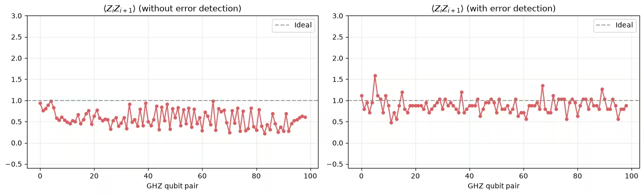
Before detection: <ZiZi+1>=  0.573749999999951
After detection: <ZiZi+1>=  0.8817377312951776

結果の解釈

2つのプロットは、100量子ビットGHZチェーンの隣接する各量子ビット・ペアについて、パリティ・チェックでポストセレクションする前と後に、シャドウ・トモグラフィーから推定された $\langle Z_i Z_{i+1}\rangle$ を示しています。

理想的なGHZ状態では、すべての最近接相関子は $1$ に等しくなります。ハードウェア上では、ノイズによって生の推定値が低下し、量子ビット間のばらつきが生じます。エラー検出後は、検出可能なエラーが少なくとも1つ発生したスナップショットが除去され、残りの推定値は分散が減少して $1$ に近づきます。これは、より clean な有効状態と整合しています。

エラー検出後の改善は、チェックが実際のエラーを検出していることと整合しています。

次のステップ

次のリソースで詳しく学べます。

おすすめ

• 量子情報の一般的な定式化
• 時空間コードを用いた低オーバーヘッドのエラー検出のチュートリアル
• Qiskit Paulice アドオンのAPIドキュメント

参考文献

• [1] Huang, H. Y., Kueng, R., & Preskill, J. (2020). Predicting many properties of a quantum system from very few measurements. Nature Physics, 16, 1050–1057.

• [2] Zhao, A., Rubin, N. C., & Miyake, A. (2021). Fermionic partial tomography via classical shadows. Phys. Rev. Lett., 127, 110504.

• [3] Low, G. H. (2022). Classical shadows of fermions with particle number symmetry. arXiv:2208.08964.

• [4] Bertoni, C., Haferkamp, J., Hinsche, M. et al. (2024). Shallow Shadows: Expectation Estimation Using Low-Depth Random Clifford Circuits. Phys. Rev. Lett., 133, 020602.

• [5] Hu, H.-Y., Gu, A., Majumder, S. et al. (2025). Demonstration of robust and efficient quantum property learning with shallow shadows. Nature Communications, 16, 2943.

• [6] Martiel, S. & Javadi-Abhari, A. (2025). Low-overhead error detection with spacetime codes. arXiv:2504.15725. © IBM Corp. 2026