スペースタイム符号による低オーバーヘッド誤り検出

使用量の見積もり: Heronプロセッサ(ibm_kingstonまたはそれに相当するもの)で4分(注: これはあくまで見積もりです。実際の実行時間は異なる場合があります。)

学習成果

• スペースタイム・パウリ・チェックがクリフォード回路の論理エラーをどのように検出するか、そしてそのシンドロームによる事後選択がサンプリングされた分布の忠実度をどのように高めるか。

• get_check_qubits、NoiseModel、add_pauli_checksを使って、qiskit-pauliceパッケージでハードウェア効率の良いチェックを自動的に見つけて挿入する方法。

• 安定化演算子をサンプリングし、チェック・シンドロームによる事後選択を行うことで、安定化状態の忠実度を推定する方法。

• IBM Quantum®ハードウェア上で完全な誤り検出ワークフローを実行し、ノイズあり忠実度と事後選択後の忠実度を比較する方法。

前提条件

• ユーティリティ・スケールの量子コンピューティングに関するハードウェアの基礎。

• クリフォードおよび安定化形式論。安定化群が純粋な安定化状態をどのように記述するかを含みます。

背景

Simon MartielとAli Javadi-Abhariによるスペースタイム符号による低オーバーヘッド誤り検出 [1]では、完全な誤り訂正とより軽量な誤り緩和の中間に位置する、クリフォード優勢な回路の論理エラーを検出する手法が紹介されています。このアイデアは、van den Bergらによるコヒーレント・パウリ・チェックによる単発誤り緩和 [2]のコヒーレント・パウリ・チェック(CPC)を基にしています。両手法とも、クリフォードの「ペイロード」回路が補助キュービットとエンタングルさせられ、特定の不変量をチェックします。補助キュービットを測定するとシンドロームが生成され、実行中にエラーが検出されたかどうかが報告されます。検出されたエラーがないサンプルのみを保持することで、事後選択率の低下と引き換えに、サンプリングされた分布の忠実度が向上します。

コヒーレント・パウリ・チェックとスペースタイム・チェックの主な違いは、測定する演算子です。コヒーレント・パウリ・チェックは時間的に局所化された高ウェイトの演算子を測定します。ヘビーヘックスのように接続性の限られたキュービット・トポロジーでは、そうしたチェックには多数のSWAPゲートが必要となり、しばしば回路が実際には実行できないほど深くなってしまいます。代わりにチェックをスペースタイム符号として実装することで、各チェックを空間と時間にわたってペイロード回路全体に分散させます。これにより、論理エラーの検出において効果的でありながら、キュービットと深さのオーバーヘッドを低く保つハードウェア効率の良い符号化が得られます。

qiskit-pauliceパッケージが行うこと

qiskit-pauliceパッケージは、これらのチェックの構築を自動化し、手作業で構築する必要がないようにします。その主な役割は、キュービットのオーバーヘッドを最小限に抑えながら誤り検出を最大化する回路内の位置に、有効なスペースタイム・パウリ・チェックを見つけて挿入することです。チェックは、その演算子がペイロード回路の論理的な動作を変えない場合に有効、少数のエンタングリング・ゲートを使う場合に低ウェイト、そのチェック自体が持ち込むノイズと比較して大部分のエラーを検出する場合に効果的とされます。このパッケージは候補となるチェックをノイズモデルに対してスコアリングし、最良のものを回路に確定します。このチュートリアルでは、次の3つのAPIメソッドを使用します。

• get_check_qubitsはバックエンドの結合マップを調べ、ターゲットと補助キュービットのペアを返します。target_qubits[i]上のチェックはancilla_qubits[i]を使用します。

• NoiseModel.from_backendは、バックエンドのベンチマーク・データからおおまかなノイズモデルを構築します。このモデルは候補となるチェックのスコアリングに使われるため、正確で学習済みのノイズモデルは必要ありません。学習済みのパウリ・リンドブラッド・モデルについては、NoiseModel.from_pauli_lindblad_mapsを参照してください。

• add_pauli_checksは回路内のチェックを見つけて挿入します。チェックの数が増加していく一連のCheckedCircuitオブジェクトを返し、各オブジェクトは測定されたビット列をシンドローム・ベクトルにマッピングするget_postselection_methodを提供します。cost引数は、チェックをスコアリングする関数を選択します(gammaは事後選択された逆ノイズ・チャネルのサンプリング・オーバーヘッド、LERは論理エラー率です)。method引数は探索戦略を選択します(windowed、genetic、windowed_genetic)。このチュートリアルでは、決定論的で再現可能なチェック選択を与えるcost="gamma"とmethod="windowed"を使用します。

安定化演算子のサンプリングから忠実度を推定する

誤り検出がどれだけうまく機能しているかを測定するために、回路が理想的に準備する安定化状態$|\psi\rangle = U|0\rangle^{\otimes n}$の忠実度を、ハードウェアが実際に出力するノイズを含む状態$\rho$に対して推定できます。純粋な安定化状態$|\psi\rangle$への射影子は、その安定化群$\mathcal{S}$の$2^n$個の要素にわたる一様平均に等しくなります。

$|\psi\rangle\langle\psi| = \frac{1}{2^n}\sum_{G \in \mathcal{S}} G.$

これを忠実度に代入すると、$\rho$の忠実度は、$\rho$に関するすべての安定化演算子$G \in \mathcal{S}$の期待値の平均として得られます。

$F = \mathrm{Tr}(\rho|\psi\rangle\langle\psi|) = \frac{1}{2^n} \sum_{G \in \mathcal{S}} \mathrm{Tr}(\rho G) = \frac{1}{2^n} \sum_{G \in \mathcal{S}} \langle G \rangle_\rho.$

より大きな問題では、すべての$2^n$個の安定化演算子を列挙するのは実行不可能なため、ランダムなサンプルから忠実度を推定できます。$\mathcal{S}$から一様ランダムに$M$個の安定化演算子$G_1, \ldots, G_M$を抽出すると、不偏推定量が得られます。

$\hat F_M = \frac{1}{M} \sum_{i=1}^M \langle G_i \rangle_\rho.$

クリフォード回路は安定化状態を準備するため、その安定化演算子のサンプリングされた期待値から直接忠実度を推定できます。このチュートリアルでは、まず小さな回路を使ってシミュレータ上でワークフローを説明し、その後、より大きく深い回路を使ってハードウェア上で同じワークフローを実行します。回路に非クリフォード演算がより多く含まれるようになると、有効なチェックの数が急速に減少するため、この手法はクリフォード優勢な回路で最も効果を発揮します。

要件

このチュートリアルを始める前に、以下がインストールされていることを確認してください。

• Qiskit SDK v2.0以降(可視化サポート付き)

• Qiskit Runtime v0.40以降(pip install qiskit-ibm-runtime)

• Qiskit Aer v0.17以降(pip install qiskit-aer)

• Qiskit Paulice(pip install qiskit-paulice)

• tqdm (pip install tqdm)

セットアップ

必要なライブラリをインポートし、インポートとして利用できないヘルパー関数を定義します。random_clifford_circuit関数はブリックワーク型のランダムなCliffordペイロードを構築し、find_check_layoutはBackendのカップリングマップを検索して、利用可能なアンシラが多く、エラーの少ないQubitパスを見つけます。learned_noise_modelはNoiseLearnerの出力をqiskit-pauliceノイズモデルに変換し、append_basis_rotationはスタビライザーが計算基底で測定されるようにCircuitを回転させ、expectationはサンプリングされたカウントからスタビライザーの期待値を計算し、cum_mean_semは継続的な忠実度推定値を追跡します。

# Added by doQumentation — required packages for this notebook
!pip install -q matplotlib numpy qiskit qiskit-aer qiskit-ibm-runtime qiskit-paulice tqdm

# Standard library imports
import random
import time

# External libraries
import matplotlib.pyplot as plt
import numpy as np
from tqdm import tqdm

# Qiskit
from qiskit import QuantumCircuit
from qiskit.quantum_info import Clifford, Pauli, PauliLindbladMap, PauliList
from qiskit.result import sampled_expectation_value
from qiskit.transpiler import generate_preset_pass_manager
from qiskit.visualization import plot_coupling_map

# Qiskit Aer
from qiskit_aer import AerSimulator
from qiskit_aer.noise import NoiseModel as AerNoiseModel
from qiskit_aer.noise import ReadoutError, depolarizing_error

# Qiskit IBM Runtime
from qiskit_ibm_runtime import NoiseLearner, QiskitRuntimeService
from qiskit_ibm_runtime import SamplerV2 as Sampler

# Qiskit Paulice
from qiskit_paulice import add_pauli_checks
from qiskit_paulice.layout import get_check_qubits
from qiskit_paulice.noise_models import NoiseModel

def random_clifford_circuit(
    num_qubits: int, depth: int, rng: np.random.Generator
) -> QuantumCircuit:
    """Brickwork random Clifford on `num_qubits`, with `depth` CZ layers."""
    qc = QuantumCircuit(num_qubits)
    qc.h(range(num_qubits))
    for d in range(depth):
        for i in range(d % 2, num_qubits - 1, 2):
            qc.cz(i, i + 1)
        for q in range(num_qubits):
            if rng.integers(0, 2):
                qc.sx(q)
            if rng.integers(0, 2):
                qc.s(q)
            if rng.integers(0, 2):
                qc.sx(q)
    return qc

def find_check_layout(
    backend,
    num_qubits: int,
    rng: np.random.Generator,
    num_trials: int = 200,
    max_gate_error: float = 0.03,
    max_readout_error: float = 0.2,
) -> list[int]:
    """Find a low-error path of `num_qubits` qubits with many available ancillas.

    Builds random self-avoiding walks on the coupling map, excluding the qubits
    and two-qubit gates whose reported errors exceed the thresholds, and keeps
    the path that offers the most target and ancilla pairs. Ties are broken by
    the lower average two-qubit gate error along the path.
    """
    target = backend.target
    gate_2q = next(
        name for name in ("cz", "ecr", "cx") if name in target.operation_names
    )

    # Collect per-edge gate errors and per-qubit readout errors
    edge_error = {}
    for qubits, props in target[gate_2q].items():
        edge = tuple(sorted(qubits))
        if props is not None and props.error is not None:
            edge_error[edge] = min(edge_error.get(edge, 1.0), props.error)
    readout_error = {
        qubit: target["measure"][(qubit,)].error
        for (qubit,) in target["measure"]
    }

    # Keep only the edges whose gate and readout errors are acceptable
    adjacency = {}
    for (q1, q2), error in edge_error.items():
        if (
            error <= max_gate_error
            and readout_error.get(q1, 1.0) <= max_readout_error
            and readout_error.get(q2, 1.0) <= max_readout_error
        ):
            adjacency.setdefault(q1, set()).add(q2)
            adjacency.setdefault(q2, set()).add(q1)

    # Random self-avoiding walks; keep the path with the most check pairs
    starts = sorted(adjacency)
    best_path = None
    best_score = (-1, float("inf"))
    for _ in range(num_trials):
        path = [starts[rng.integers(len(starts))]]
        while len(path) < num_qubits:
            options = sorted(adjacency[path[-1]] - set(path))
            if not options:
                break
            path.append(options[rng.integers(len(options))])
        if len(path) < num_qubits:
            continue
        num_pairs = len(get_check_qubits(backend.coupling_map, path)[0])
        mean_error = float(
            np.mean(
                [edge_error[tuple(sorted(e))] for e in zip(path, path[1:])]
            )
        )
        if num_pairs > best_score[0] or (
            num_pairs == best_score[0] and mean_error < best_score[1]
        ):
            best_path, best_score = path, (num_pairs, mean_error)

    if best_path is None:
        raise RuntimeError(
            "No connected low-error path found. Relax the error thresholds."
        )
    return best_path

def learned_noise_model(layer_errors, layout: list[int]) -> NoiseModel:
    """Build a `NoiseModel` from `NoiseLearner` results.

    `NoiseLearner` reports one `PauliLindbladError` per entangling layer, whose
    generators are indexed against that layer's own physical qubits, while
    `NoiseModel.from_pauli_lindblad_maps` expects `PauliLindbladMap`s indexed the
    way `NoiseModel.from_backend` indexes them: by position in `layout`. This
    translates between the two and drops generators that fall outside `layout`.
    """
    phys_to_virt = {phys: virt for virt, phys in enumerate(layout)}
    maps = []
    for layer in layer_errors:
        if layer.error is None:
            continue
        terms = []
        for pauli, rate in zip(
            layer.error.generators, layer.error.rates, strict=True
        ):
            label, indices = [], []
            for local, phys in enumerate(layer.qubits):
                x, z = bool(pauli.x[local]), bool(pauli.z[local])
                if not (x or z):
                    continue
                if phys not in phys_to_virt:
                    break  # generator reaches outside the layout, so skip it
                label.append("Y" if x and z else "X" if x else "Z")
                indices.append(phys_to_virt[phys])
            else:
                if label:
                    terms.append(
                        ("".join(label), tuple(indices), float(rate))
                    )
        # Each map needs a 2-qubit generator to define an entangling layer
        if any(len(t[1]) == 2 for t in terms):
            maps.append(
                PauliLindbladMap.from_sparse_list(
                    terms, num_qubits=len(layout)
                )
            )
    if not maps:
        raise RuntimeError(
            "No usable layer errors. Check that the learner ran on this layout."
        )
    return NoiseModel.from_pauli_lindblad_maps(maps)

def append_basis_rotation(
    circuit: QuantumCircuit, pauli: Pauli
) -> QuantumCircuit:
    """Strip measurements, append basis rotations for `pauli`, and re-measure."""
    out = circuit.remove_final_measurements(inplace=False)
    for q in range(pauli.num_qubits):
        if pauli.x[q]:
            if pauli.z[q]:
                out.sdg(q)
            out.h(q)
    out.measure_all()
    return out

def expectation(counts: dict, pauli: Pauli) -> float:
    """Expectation value of `pauli` from counts measured in the Z basis.

    Pads with identity on any qubits beyond the support of `pauli`, such as the
    check ancillas that appear in the postselected counts.
    """
    if not counts:
        return float("nan")
    n = pauli.num_qubits
    sign = -1 if int(pauli.phase) % 4 == 2 else 1
    total = len(next(iter(counts)))
    label = "".join(
        "Z" if q < n and (pauli.x[q] or pauli.z[q]) else "I"
        for q in range(total - 1, -1, -1)
    )
    return sign * sampled_expectation_value(counts, label)

def cum_mean_sem(values: np.ndarray):
    """Cumulative mean and standard error of the mean, ignoring NaNs."""
    valid = ~np.isnan(values)
    total = np.cumsum(np.where(valid, values, 0.0))
    total_sq = np.cumsum(np.where(valid, values**2, 0.0))
    count = np.maximum(np.cumsum(valid).astype(float), 1)
    mean = total / count
    sem = np.sqrt(np.maximum(total_sq / count - mean**2, 0) / count)
    return np.where(np.cumsum(valid) > 0, mean, np.nan), sem

小規模シミュレーター例

このセクションでは、ノイズのあるシミュレーター上で全体のワークフローを説明します。Backendのベンチマークデータを使用してQubitレイアウトとノイズモデルを選択し、チェックを自動的に見つけ、サンプリングされた分布に対するポストセレクションを使用して忠実度の改善を示します。

ステップ1: 古典入力を量子問題にマッピングする

ペイロードCircuitは浅い一次元のブリックワーク型ランダムCliffordCircuitです。CircuitがCliffordであるため、サンプリングされたスタビライザーの期待値から直接忠実度を推定できるスタビライザー状態を準備します。次のステップでチェックを視覚化しやすいように、浅いCircuitから始めます。

num_qubits = 12
depth = 4
seed = 1764
rng = np.random.default_rng(seed)
np.random.seed(seed)

circuit = random_clifford_circuit(num_qubits, depth, rng)
circuit.measure_all()
circuit.draw("mpl", fold=-1, scale=0.6)

ステップ2: 量子ハードウェア実行向けに最適化する

Circuitをハードウェアにマッピングすることで、物理Qubitレイアウト、候補チェックをスコアリングするノイズモデル、そしてチェック自体が設定されます。

まず、Backendを選択し、セットアップのセクションで定義したfind_check_layoutヘルパーを使用してそのカップリングマップから一次元のQubitレイアウトを検索します。このヘルパーは、エラー率が最も高いGateと読み出しを避けるランダムな自己回避ウォークを構築し、ターゲットとアンシラのペアを最も多く提供するパスを保持します。検索はBackend自体から接続性とエラーデータを読み取るため、同じコードはどのIBM Quantum QPUでも実行できます。次にget_check_qubits関数がターゲットとアンシラのペアを返します。target_qubits[i]に対するチェックはancilla_qubits[i]を使用します。

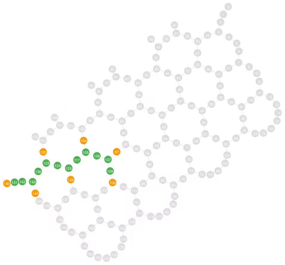
以下のカップリンググラフでは、緑色のQubitがペイロードQubitで、オレンジ色のQubitがチェックを実装するアンシラです。隣接するアンシラを持つQubitはチェックのターゲットQubitとして使用されます。

service = QiskitRuntimeService()
backend = service.least_busy(operational=True, simulator=False)

print(f"Backend: {backend.name}")

# Search for a low-error path, then pair each target qubit with a neighboring ancilla
layout = find_check_layout(backend, num_qubits, rng)
target_qubits, ancilla_qubits = get_check_qubits(backend, layout)
num_checks = len(target_qubits)

print(f"Target qubits:  {target_qubits}")
print(f"Ancilla qubits: {ancilla_qubits}")
plot_coupling_map(
    num_qubits=backend.num_qubits,
    qubit_coordinates=getattr(
        backend.configuration(), "qubit_coordinates", None
    ),
    coupling_map=backend.configuration().coupling_map,
    figsize=(12, 12),
    qubit_color=[
        "#4CAF50"
        if i in set(layout)
        else "#FF9800"
        if i in set(ancilla_qubits)
        else "#DDDDDD"
        for i in backend.coupling_map.graph.node_indices()
    ],
    qubit_size=220,
    line_width=2,
    font_size=90,
)

Backend: ibm_boston
Target qubits:  [105, 107, 108, 123, 125, 141, 143]
Ancilla qubits: [104, 97, 109, 122, 126, 140, 144]

Backendとレイアウトを選択したら、ペイロードを命令セットアーキテクチャ(ISA)Circuitにトランスパイルします。レイアウトを設定し、Gateを Backend のネイティブGateセットに変換するだけで十分です。

pm = generate_preset_pass_manager(
    optimization_level=0, backend=backend, initial_layout=layout
)
circuit_isa = pm.run(circuit)
circuit_isa.draw("mpl", fold=-1, scale=0.6)

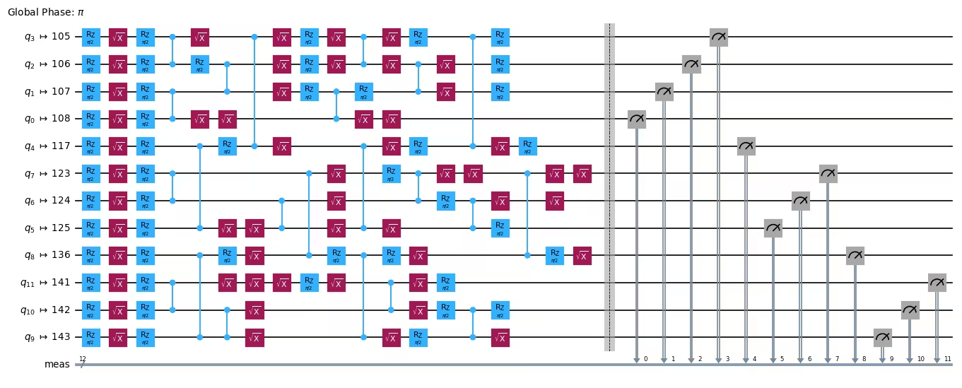
次に、BackendのGateと読み出しのノイズが実行にどのように影響するかをモデル化します。ノイズモデルは、Circuit内のどこでチェックが最も多くのエラーを捕捉するかを決定します。より正確なモデルは検出精度を向上させますが、通常はQPUをサンプリングしてモデルを学習する必要はありません。以下のモデルは、qiskit-ibm-runtimeのベンチマークデータからGateと読み出しノイズの均一な脱分極チャネルを推定します。

noise_model = NoiseModel.from_backend(
    backend, layout, uniform_gate_noise=True
)
print(noise_model)

NoiseModel(gate_noise=0.001079865281450939, readout_noise=0.006001790364583333, idling_noise=None)

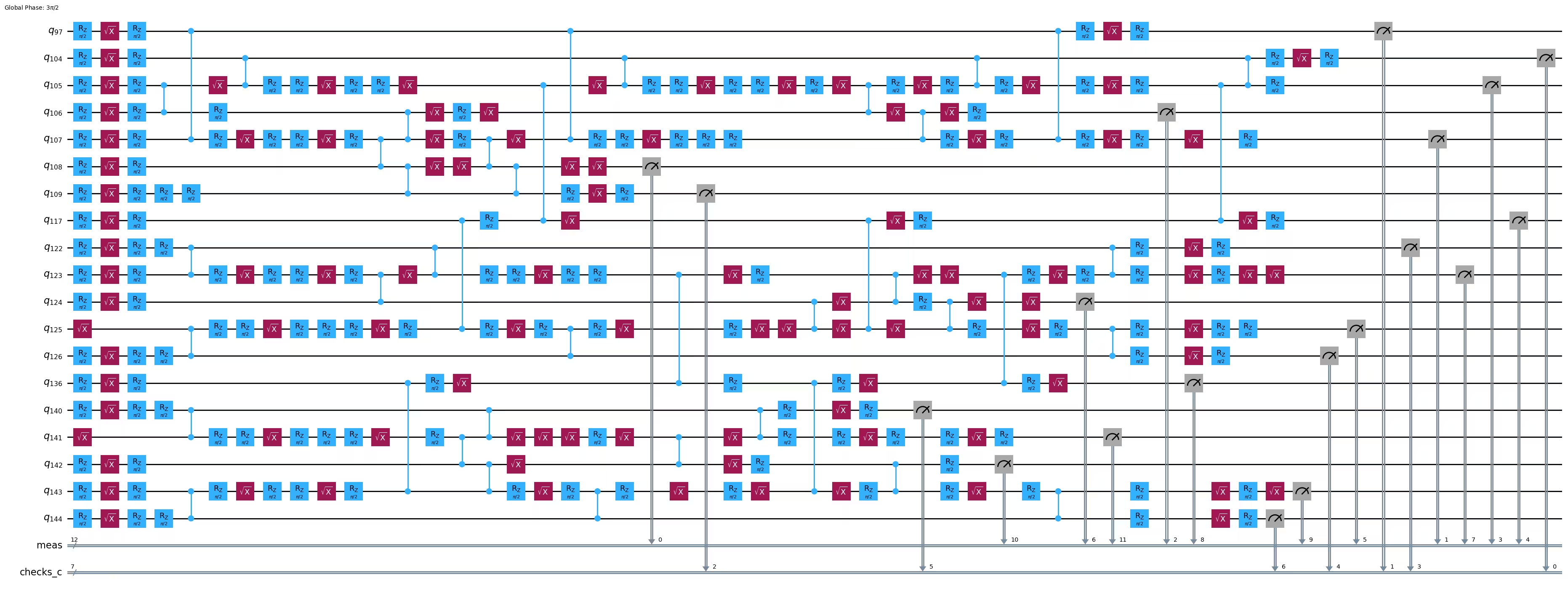
次に、Circuitにチェックを追加します。add_pauli_checks関数は、Cliffordペイロード、ターゲットQubitのリスト、そしてノイズモデルを受け取ります。ancilla_qubits引数は、どの物理アンシラを各ターゲットとペアにするかを関数に伝えます。チェックはターゲットQubitが現れる順序で追加されるため、チェック済みCircuitの最終レイアウトはlayout + ancilla_qubitsになります。チェック数が少ない(i個)出力Circuitを実行するには、最終レイアウトはlayout + ancilla_qubits[:i]になります。

add_pauli_checksの出力は、チェックなしからすべてのターゲットQubitに1つのチェックが付くまで、チェックの数が増加していくCircuitのシーケンスです。可視化により、チェックが指定されたターゲットとアンシラのペアを使用していることが確認できます。良いチェックの見つけ方の詳細については、参考文献[1]の補足情報のセクションIIからIVを参照してください。

checked = add_pauli_checks(
    circuit_isa,
    target_qubits,
    noise_model,
    ancilla_qubits=ancilla_qubits,
    cost="gamma",
    method="windowed",
    seed=seed,
)

print(f"Physical layout of payload and ancillas: {layout + ancilla_qubits}")
print("Checked circuit:")
checked[-1].circuit.draw("mpl", fold=-1, idle_wires=False)

Physical layout of payload and ancillas: [108, 107, 106, 105, 117, 125, 124, 123, 136, 143, 142, 141, 104, 97, 109, 122, 126, 140, 144]
Checked circuit:

ステップ3: Qiskitプリミティブを使用して実行する

Gateノイズの影響を見えるようにするために、ペイロードの深さを増やし、そのスタビライザーのサブセットをサンプリングします。各スタビライザーは一般的に他のスタビライザーとQubit単位で可換ではないため、1つのチェックセットは2つの異なるスタビライザーには有効ではありません。スタビライザーを可換なセットにグループ化する代わりに、各スタビライザーに対して独立に良いチェックセットを見つけます。スタビライザーを一様ランダムにサンプリングすることで、偏りのない忠実度推定値が得られます。

より深いCircuitを構築し、そのスタビライザーのランダムサンプルを取得します。

depth = 24
num_stabilizers = 20
num_shots = 1_000

circuit = random_clifford_circuit(num_qubits, depth, rng)

# Build the full stabilizer group, then sample from it uniformly at random
circ_no_meas = circuit.remove_final_measurements(inplace=False)
stabilizer_group = PauliList([Pauli("I" * num_qubits)])
for generator in (
    Pauli(label) for label in Clifford(circ_no_meas).to_labels(mode="S")
):
    stabilizer_group = stabilizer_group + stabilizer_group.compose(generator)

keep = np.where(
    stabilizer_group.x.any(axis=1) | stabilizer_group.z.any(axis=1)
)[0]
chosen = np.random.default_rng(seed).choice(
    keep, size=min(num_stabilizers, len(keep)), replace=False
)
stabilizers = [stabilizer_group[int(i)] for i in chosen]

two_qubit_depth = circuit.depth(lambda x: x.operation.num_qubits == 2)
print(
    f"Sampled {len(stabilizers)} stabilizers of a {circuit.num_qubits}-qubit "
    f"circuit with two-qubit depth {two_qubit_depth}: "
    f"{{{stabilizers[0]}, {stabilizers[1]}, ...}}"
)

Sampled 20 stabilizers of a 12-qubit circuit with two-qubit depth 24: {ZXIIXZYYXIZZ, XXXYIIZYXIII, ...}

サンプリングされた各スタビライザーについて、スタビライザーが計算基底で測定されるようにCircuitを回転させ、それをBackendにトランスパイルし、良いチェックセットを見つけます。ターゲットとアンシラのペアは各スタビライザーごとに一緒にシャッフルされるため、各ターゲットはそのアンシラを保持します。チェックは、ターゲットQubitが与えられた順序で逐次コミットされ、コミットされたチェックはチェックが追加されても変更されないことに注意してください。

noisy_circuits = []
checked_circuits = []
depths_2q = []
t0 = time.time()
for i, pauli in enumerate(tqdm(stabilizers)):
    noisy_circuits.append(pm.run(append_basis_rotation(circuit, pauli)))
    # Shuffle target and ancilla pairs together so each target keeps its ancilla
    targets, ancillas = zip(
        *random.sample(
            list(zip(target_qubits, ancilla_qubits, strict=True)),
            k=len(target_qubits),
        ),
        strict=True,
    )
    checked_circuits.append(
        add_pauli_checks(
            noisy_circuits[-1],
            list(targets),
            noise_model,
            ancilla_qubits=list(ancillas),
            cost="gamma",
            method="windowed",
            seed=seed + 1 + i,
        )
    )
    depths_2q.append(
        checked_circuits[-1][-1].circuit.depth(lambda x: len(x.qubits) == 2)
    )

print(
    f"Added {num_checks} checks to {len(stabilizers)} circuits "
    f"in {(time.time() - t0):.0f}s."
)
print(
    f"On average, two-qubit depth increased from "
    f"{circuit.depth(lambda x: len(x.qubits) == 2)} to {int(np.mean(depths_2q))} "
    f"when adding {num_checks} checks."
)

100%|██████████| 20/20 [00:15<00:00,  1.29it/s]

Added 7 checks to 20 circuits in 15s.
On average, two-qubit depth increased from 24 to 33 when adding 7 checks.

Qiskit Aerを使用して、ベアのペイロードとチェック済みCircuitをサンプリングします。シミュレーターはチェックをスコアリングしたのと同じ脱分極モデルを使用するため、チェックが対象とするノイズは、シミュレーターが適用するノイズと同じです。

aer_nm = AerNoiseModel()
aer_nm.add_all_qubit_quantum_error(
    depolarizing_error(noise_model.gate_noise, 2), ["cz"]
)
p = noise_model.readout_noise
aer_nm.add_all_qubit_readout_error(ReadoutError([[1 - p, p], [p, 1 - p]]))
noisy_sim = AerSimulator(method="stabilizer", noise_model=aer_nm)

counts = []
for i, checked_circ_result in enumerate(tqdm(checked_circuits)):
    noisy_counts = (
        noisy_sim.run(
            noisy_circuits[i], shots=num_shots, seed_simulator=seed * i + 1
        )
        .result()
        .get_counts()
    )
    checked_counts_per_variant = []
    for k, ck in enumerate(checked_circ_result):
        variant_counts = (
            noisy_sim.run(
                ck.circuit, shots=num_shots, seed_simulator=seed * i + 2 + k
            )
            .result()
            .get_counts()
        )
        checked_counts_per_variant.append(variant_counts)
    counts.append((noisy_counts, checked_counts_per_variant))

100%|██████████| 20/20 [00:17<00:00,  1.13it/s]

ステップ4: 後処理を行い、目的の古典形式で結果を返す

各チェックは、1つのアンシラと1つのターゲットの間のもつれGateを使用します。アンシラは$|0\rangle$から始まるため、$Z_\text{anc}$はその入力を安定化します。$Z_\text{anc}$をチェック済みCircuitを通じて前方に伝播させると、出力上のPauli演算子が得られ、その非単位項がチェックのサポートを定義します。チェックのサポート内のビットが偶数パリティを持つとき、チェックは合格します。サンプルは、すべてのチェックが合格した場合にのみ保持されます。

各CheckedCircuitのget_postselection_methodは、測定されたビット列をシンドロームベクトルにマッピングする関数を返します。すべてのチェックについてシンドロームがゼロであるサンプルを保持し、残りを破棄します。以下のチャートは、チェックを追加するほどポストセレクション率が低下することを示しています。ポストセレクション率が低いほど、目標精度に到達するためにより多くのショットが必要になるため、検出能力とサンプリングコストの間にトレードオフがあります。この率は収束するように見え、追加のチェックが寄与する検出能力が小さくなっていくことを示しています。

rate_per_variant = []
kept_per_stab = []
for i, (_, checked_counts_per_variant) in enumerate(counts):
    rates = []
    kept_at_num_checks = None
    for k, variant_counts in enumerate(checked_counts_per_variant):
        ps_fn = checked_circuits[i][k].get_postselection_method()
        kept = {
            bs: n for bs, n in variant_counts.items() if not ps_fn(bs).any()
        }
        rates.append(sum(kept.values()) / num_shots)
        if k == num_checks:
            kept_at_num_checks = kept
    rate_per_variant.append(rates)
    kept_per_stab.append(kept_at_num_checks)

max_len = max(len(s) for s in rate_per_variant)
rates_arr = np.full((len(rate_per_variant), max_len), np.nan)
for i, s in enumerate(rate_per_variant):
    rates_arr[i, : len(s)] = s
ks = np.arange(max_len)

fig, ax = plt.subplots(figsize=(8, 4))
ax.plot(ks, rates_arr.T, color="#ff8c00", alpha=0.15, linewidth=1)
ax.plot(
    ks,
    np.nanmedian(rates_arr, axis=0),
    color="black",
    linewidth=1,
    linestyle="--",
    label="median",
)
ax.set_xlabel("Checks committed")
ax.set_ylabel("Postselection rate")
ax.set_ylim((0, 1.05))
ax.set_title(
    f"Per-stabilizer postselection rate ({len(rates_arr)} stabilizers)"
)
ax.legend()
ax.grid(True, alpha=0.3)
plt.tight_layout()
plt.show()

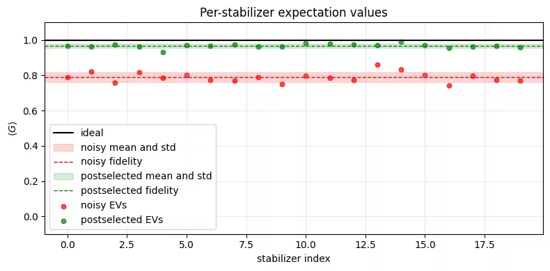
ここで、ベアなノイズのある状態の忠実度とポストセレクション後の状態の忠実度を比較します。エラーが検出されなかったサンプルのみをポストセレクションすることで、すべてのスタビライザーの期待値、ひいては推定忠実度が向上します。ポストセレクションされた値は生の値よりも少ないサンプル数を使用していますが、期待値はより正確で、サンプリングされた分散はより小さくなっています。また、平均ポストセレクション率がノイズのある忠実度に近いことにも注目してください。これは、チェックがほぼすべての誤ったサンプルを検出する場合に期待される結果です。すべてのチェックに合格したサンプルの割合は、エラーのないサンプルの割合、つまりノイズのある状態の忠実度に近づきます。

results = []
for i, ((noisy_counts, _), kept) in enumerate(
    zip(counts, kept_per_stab, strict=True)
):
    results.append(
        (
            expectation(noisy_counts, stabilizers[i]),
            expectation(kept, stabilizers[i]),
            sum(kept.values()) / num_shots,
        )
    )

fidelity_noisy = float(np.nanmean([r[0] for r in results]))
fidelity_postsel = float(np.nanmean([r[1] for r in results]))
psr = float(np.mean([r[2] for r in results]))
print(
    f"ideal fidelity:          1.0\n"
    f"noisy fidelity:          {fidelity_noisy:.4f}\n"
    f"postselected fidelity:   {fidelity_postsel:.4f}\n"
    f"mean postselection rate: {psr:.3f}"
)

evs_ideal = np.ones(len(results))
evs_noisy = np.array([r[0] for r in results])
evs_post = np.array([r[1] for r in results])
idx = np.arange(len(results))

def strip(ax, ys, color, label):
    m, s = np.nanmean(ys), np.nanstd(ys)
    ax.axhspan(
        m - s, m + s, color=color, alpha=0.15, label=f"{label} mean and std"
    )
    ax.axhline(
        m, color=color, linewidth=1, linestyle="--", label=f"{label} fidelity"
    )

fig, ax = plt.subplots(figsize=(8, 4))
ax.axhline(np.nanmean(evs_ideal), color="black", linewidth=1.5, label="ideal")
strip(ax, evs_noisy, "red", "noisy")
strip(ax, evs_post, "green", "postselected")
ax.scatter(idx, evs_noisy, color="red", s=22, alpha=0.7, label="noisy EVs")
ax.scatter(
    idx,
    evs_post,
    color="green",
    s=22,
    alpha=0.7,
    label="postselected EVs",
)
ax.set_xlabel("stabilizer index")
ax.set_ylabel(r"$\langle G \rangle$")
ax.set_ylim((-0.1, 1.1))
ax.set_title("Per-stabilizer expectation values")
ax.legend(loc="lower left")
ax.grid(True, alpha=0.3)
plt.tight_layout()
plt.show()

M = np.arange(1, len(results) + 1)
fig, ax = plt.subplots(figsize=(8, 4))
for ys, color, label in [
    (evs_ideal, "black", "ideal"),
    (evs_noisy, "red", "noisy"),
    (evs_post, "green", "postselected"),
]:
    cm, sem = cum_mean_sem(ys)
    ax.plot(M, cm, color=color, linewidth=1.5, label=label)
    ax.fill_between(M, cm - sem, cm + sem, color=color, alpha=0.15)
ax.set_xlabel("number of stabilizers averaged")
ax.set_ylabel("running fidelity estimate")
ax.set_title("Fidelity convergence versus number of stabilizers")
ax.legend()
ax.grid(True, alpha=0.3)
plt.tight_layout()
plt.show()

ideal fidelity:          1.0
noisy fidelity:          0.7899
postselected fidelity:   0.9679
mean postselection rate: 0.780

ガンマスコアは、モデル化されたノイズチャネルのうち、チェックによって検出されずに残る割合を報告します。ガンマスコアをコミットされたチェックの数に対してプロットすると、チェックが追加されるにつれて検出能力がどのように向上するかがわかります。値1.0は、チェックがモデル化されたノイズをすべて捕捉することを意味します。チェックがコミットされるにつれて曲線は1.0に向かって下降し、各追加チェックが残りの未検出エラーの一部を捕捉していることを示しています。

stab_scores = [
    [variant.cost for variant in checked_circ_result]
    for checked_circ_result in checked_circuits
]
max_len = max(len(s) for s in stab_scores)
scores = np.full((len(stab_scores), max_len), np.nan)
for i, s in enumerate(stab_scores):
    scores[i, : len(s)] = s
ks = np.arange(max_len)

fig, ax = plt.subplots(figsize=(8, 4))
ax.plot(ks, scores.T, color="#4682b4", alpha=0.15, linewidth=1)
ax.plot(
    ks,
    np.nanmedian(scores, axis=0),
    color="black",
    linewidth=1,
    linestyle="--",
    label="median",
)
ax.set_xlabel("Checks committed")
ax.set_ylabel("Gamma")
ax.set_yscale("log")
ax.set_title(f"Per-stabilizer gamma curves ({len(scores)} stabilizers)")
ax.legend()
ax.grid(True, alpha=0.3, which="both")
plt.tight_layout()
plt.show()

大規模ハードウェア例

同じワークフローが、より大きく深いペイロードを持つハードウェア上で実行されます。このセクションでは、シミュレーター例と同じBackendを再利用しますが、独自のターゲットとアンシラのペアおよびパスマネージャーを持つ新しい20QubitレイアウトCircuitを構築し、Circuitを1つのジョブでQPUに送信します。この規模では、ほとんどのショットが少なくとも1つのチェックを発生させるため、ポストセレクション率は低く、各Circuitは十分なサンプルが残るように大きなショット予算を必要とします。そのため、この例ではその予算を少数のサンプリングされたスタビライザーに集中させます。これは依然として偏りのない忠実度推定値ですが、多くのスタビライザーの平均を取るシミュレーター例よりも粗いものです。

シミュレーター例と比較して変わる点が1つあります。キャリブレーションデータから均一な脱分極チャネルを推定する代わりに、このセクションではNoiseLearnerを使用してノイズモデルを学習し、NoiseModel.from_pauli_lindblad_mapsを使用してその結果からqiskit-pauliceモデルを構築します。学習されたPauli-Lindbladモデルは、すべてのエッジが同じようにノイズが多いと仮定するのではなく、この特定のレイアウト上のノイズの空間的構造を捉えるため、チェックの配置はQPUに影響を与えるノイズにより類似したノイズに対してスコアリングされます。ノイズの学習にはQPUのサンプリングが必要であり、全体のQPUサンプリング予算で考慮する必要があります。

以下のパラメーターは、Qubitの数、深さ、スタビライザーの数、ショットの数を設定します。hw_num_shotsをポストセレクション率の逆数に応じてスケールしてください。3%の率では、40,000ショットで1Circuitあたりおよそ1,200のポストセレクションされたサンプルが残ります。hw_num_stabilizersを増やすと、ジョブあたりのCircuitが増えるという代償を払ってより精密な忠実度推定が得られ、各Circuitは同じショット予算を必要とします。

ステップ1-4(1つのコードブロックに圧縮)

以下のセルは、シミュレーター例と同じ4つのステップを実行します。より大きなペイロードを構築していくつかのスタビライザーをサンプリングし(ステップ1)、レイアウトを選択し、その上でノイズモデルを学習し、各スタビライザーに対して完全にチェックされたCircuitを見つけ(ステップ2)、ベアとチェック済みの両方のCircuitを含む1つのSamplerジョブを送信し(ステップ3)、チェック済みのカウントをポストセレクションして、スタビライザーごとおよび平均でノイズありと ポストセレクション後の忠実度推定値を比較します(ステップ4)。この規模では、シミュレーター例のようにスタビライザー群全体を列挙することは不可能であるため、このセルはスタビライザーのランダムなサブセットをサブサンプリングして忠実度の推定値を計算します。

ここではステップ2がシミュレーター例よりも多くのことを行うことに注意してください。ノイズモデルの学習は、Samplerジョブの前に独自のNoiseLearnerジョブを送信するため、このセルは合計で2つのジョブを実行します。これらには後で見つけられるようにTUT_ASPC_LEARNとTUT_ASPCというタグが付けられています。ジョブへのタグ付けの詳細については、ジョブタグによる整理と検索を参照してください。

# -------------------------Step 1: build a larger payload and sample stabilizers-------------------------
hw_num_qubits = 20
hw_depth = 36
hw_num_stabilizers = 10
hw_num_shots = 40_000

hw_circuit = random_clifford_circuit(hw_num_qubits, hw_depth, rng)
hw_no_meas = hw_circuit.remove_final_measurements(inplace=False)

# Enumerating all 2^n stabilizers is infeasible at this size, so draw each
# stabilizer by composing a random subset of the group generators
hw_generators = [
    Pauli(label) for label in Clifford(hw_no_meas).to_labels(mode="S")
]
sample_rng = np.random.default_rng(seed)
hw_stabilizers = []
while len(hw_stabilizers) < hw_num_stabilizers:
    mask = sample_rng.integers(0, 2, hw_num_qubits).astype(bool)
    if not mask.any():
        continue  # skip the identity
    stabilizer = Pauli("I" * hw_num_qubits)
    for generator, chosen in zip(hw_generators, mask, strict=True):
        if chosen:
            stabilizer = stabilizer.compose(generator)
    hw_stabilizers.append(stabilizer)

# -------------------------Step 2: find a 20-qubit layout, learn its noise, and add checks-------------------------
# A single bad coupler or bad-readout qubit on the path drags every
# stabilizer down, so search harder and with tighter error thresholds
hw_layout = find_check_layout(
    backend,
    hw_num_qubits,
    rng,
    num_trials=500,
    max_gate_error=0.015,
    max_readout_error=0.05,
)
hw_target_qubits, hw_ancilla_qubits = get_check_qubits(backend, hw_layout)
hw_pm = generate_preset_pass_manager(
    optimization_level=0, backend=backend, initial_layout=hw_layout
)
print(f"Layout with {len(hw_target_qubits)} check pairs: {hw_layout}")

# ----- learn a Pauli-Lindblad noise model on this layout -----
# The simulator example scored checks against a uniform depolarizing channel
# inferred from calibration data. Here, learn the noise instead: NoiseLearner
# runs its own job on the QPU and returns a Pauli-Lindblad channel per unique
# entangling layer, so the checks are placed against the noise this layout
# actually has, including its spatial structure. All the sampled stabilizers
# share the same entangling layers and differ only in their final basis
# rotation, so learning on the bare payload covers all of them.
learner = NoiseLearner(
    mode=backend,
    options={
        "max_layers_to_learn": 4,
        "num_randomizations": 32,
        "shots_per_randomization": 128,
        "environment": {"job_tags": ["TUT_ASPC_LEARN"]},
    },
)
learner_job = learner.run([hw_pm.run(hw_circuit)])
print(f"Submitted noise-learner job {learner_job.job_id()}")
hw_layer_errors = learner_job.result().data

# To see how much the learned model helps, swap the next line for the
# simulator example's uniform model - a one-line change:
# hw_noise_model = NoiseModel.from_backend(backend, hw_layout, uniform_gate_noise=True)
hw_noise_model = learned_noise_model(hw_layer_errors, hw_layout)
# NoiseLearner characterizes gate noise only, so keep the readout estimate
# from calibration data rather than leaving it unset
hw_noise_model.readout_noise = NoiseModel.from_backend(
    backend, hw_layout, uniform_gate_noise=True
).readout_noise
print(
    f"Learned {len(hw_layer_errors)} layers; "
    f"readout noise {hw_noise_model.readout_noise:.5f}"
)

# ----- add the fully checked circuit per stabilizer -----
hw_noisy_circuits = []
hw_checked_circuits = []
for i, pauli in enumerate(tqdm(hw_stabilizers)):
    bare = hw_pm.run(append_basis_rotation(hw_circuit, pauli))
    hw_noisy_circuits.append(bare)
    variants = add_pauli_checks(
        bare,
        hw_target_qubits,
        hw_noise_model,
        ancilla_qubits=hw_ancilla_qubits,
        cost="gamma",
        method="windowed",
        seed=seed + 1 + i,
    )
    hw_checked_circuits.append(variants[-1])  # keep the fully checked circuit

# -------------------------Step 3: submit one Sampler job with the bare and checked circuits-------------------------
sampler = Sampler(mode=backend)
sampler.options.default_shots = hw_num_shots
sampler.options.environment.job_tags = ["TUT_ASPC"]

pubs = hw_noisy_circuits + [cc.circuit for cc in hw_checked_circuits]
job = sampler.run(pubs)
print(f"Submitted job {job.job_id()} with {len(pubs)} circuits")

# -------------------------Step 4: postselect and compare fidelity-------------------------
result = job.result()
n_stab = len(hw_stabilizers)

hw_results = []
for i in range(n_stab):
    noisy_counts = result[i].join_data().get_counts()
    checked_counts = result[n_stab + i].join_data().get_counts()
    ps_fn = hw_checked_circuits[i].get_postselection_method()
    kept = {bs: c for bs, c in checked_counts.items() if not ps_fn(bs).any()}
    hw_results.append(
        (
            expectation(noisy_counts, hw_stabilizers[i]),
            expectation(kept, hw_stabilizers[i]),
            sum(kept.values()) / sum(checked_counts.values()),
        )
    )

hw_fidelity_noisy = float(np.nanmean([r[0] for r in hw_results]))
hw_fidelity_postsel = float(np.nanmean([r[1] for r in hw_results]))
hw_psr = float(np.mean([r[2] for r in hw_results]))
print(
    f"noisy fidelity estimate:        {hw_fidelity_noisy:.4f}\n"
    f"postselected fidelity estimate: {hw_fidelity_postsel:.4f}\n"
    f"mean postselection rate:        {hw_psr:.4f} "
    f"(~{int(round(hw_psr * hw_num_shots))} kept shots per circuit)"
)

# Per-stabilizer breakdown. The postselection rate varies from stabilizer to
# stabilizer, so a stabilizer whose postselected value barely moves is usually
# one whose checks rejected little; the kept-shot count says how much of the
# gap is statistics rather than signal.
print("\nper-stabilizer results:")
print(
    f"{'idx':>3}  {'noisy':>8}  {'postsel':>8}  {'psr':>7}  {'kept shots':>10}"
)
for i, (noisy, post, psr_i) in enumerate(hw_results):
    print(
        f"{i:>3}  {noisy:>8.4f}  {post:>8.4f}  {psr_i:>7.4f}  "
        f"{int(round(psr_i * hw_num_shots)):>10}"
    )

hw_noisy = np.array([r[0] for r in hw_results])
hw_post = np.array([r[1] for r in hw_results])
idx = np.arange(n_stab)

fig, ax = plt.subplots(figsize=(9, 4))
ax.axhline(1.0, color="black", linewidth=1.5, label="ideal")
strip(ax, hw_noisy, "red", "noisy")
strip(ax, hw_post, "green", "postselected")
ax.scatter(idx, hw_noisy, color="red", s=22, alpha=0.7, label="noisy EVs")
ax.scatter(
    idx,
    hw_post,
    color="green",
    s=22,
    alpha=0.7,
    label="postselected EVs",
)
ax.set_xlabel("stabilizer index")
ax.set_ylabel(r"$\langle G \rangle$")
ax.set_ylim((-0.1, 1.1))
ax.set_xticks(idx)
ax.set_title("Per-stabilizer expectation values on hardware")
# Outside the axes so it cannot hide a data point
ax.legend(loc="center left", bbox_to_anchor=(1.02, 0.5), frameon=False)
ax.grid(True, alpha=0.3)
plt.tight_layout()
plt.show()

Layout with 11 check pairs: [153, 152, 151, 138, 131, 130, 129, 118, 109, 110, 111, 98, 91, 90, 89, 78, 69, 70, 71, 58]
Submitted noise-learner job d9f4mncjeosc73fjfmkg

Learned 4 layers; readout noise 0.00470

100%|██████████| 10/10 [01:01<00:00,  6.18s/it]

Submitted job d9f4s04jeosc73fjftkg with 20 circuits
noisy fidelity estimate:        0.3685
postselected fidelity estimate: 0.6869
mean postselection rate:        0.2851 (~11404 kept shots per circuit)

per-stabilizer results:
idx     noisy   postsel      psr  kept shots
  0    0.3769    0.6918   0.3247       12987
  1    0.3745    0.6760   0.2999       11995
  2    0.3659    0.6389   0.3549       14196
  3    0.3821    0.7060   0.2660       10641
  4    0.3653    0.7475   0.2531       10124
  5    0.3752    0.7022   0.2698       10791
  6    0.3508    0.7144   0.2711       10842
  7    0.3485    0.7087   0.2381        9523
  8    0.3825    0.6289   0.2928       11711
  9    0.3630    0.6549   0.2808       11232

この規模のCircuitでは、ほとんどのサンプルに少なくとも1つの検出されたエラーが含まれているため、ポストセレクション率は小さく、ポストセレクションはほとんどのショットを破棄します。すべてのチェックに合格したサンプルは、ベアのCircuitよりもはるかに優れた期待値を与え、スタビライザーごとの値はノイズのあるベースラインからきれいに分離します。忠実度推定を精密にするには、同じCircuitあたりのショット予算でより多くのスタビライザーをサンプリングします。ポストセレクション率を上げるには、Circuitの深さを減らすか、コミットするチェック数を減らします。より大きなペイロードに拡張するには、ショット予算をポストセレクション率の逆数でスケールします。

次のステップ

推奨事項

この内容に興味を持たれた方には、以下の資料もお勧めします。

• 量子誤り訂正の入門として、反復コードのチュートリアル。

• 完全なチェック検索APIについてはqiskit-pauliceドキュメントを、ソースコードについてはパッケージのGitHubリポジトリを参照してください。

• チェックの背後にある理論については、論文Low-overhead error detection with spacetime codesを参照してください。

参考文献

• [1] Martiel, S., & Javadi-Abhari, A. (2025). Low-overhead error detection with spacetime codes. arXiv preprint arXiv:2504.15725.

• [2] van den Berg, E., Bravyi, S., Gambetta, J. M., Jurcevic, P., Maslov, D., & Temme, K. (2023). Single-shot error mitigation by coherent Pauli checks. Physical Review Research, 5(3), 033193.