動的回路を用いたキックドイジングハミルトニアンのシミュレーション

使用量の目安: Heron r3 プロセッサで約7.5分（注意: これはあくまで推定値です。実際の実行時間は異なる場合があります。） 動的回路とは、古典的なフィードフォワードを伴う回路のことです。言い換えると、回路の途中で測定を行い、その古典的な出力に基づいて条件付きの量子操作を決定する古典的な論理演算を実行する回路です。このチュートリアルでは、六角格子上のスピンに対してキックドイジングモデルをシミュレーションし、動的回路を使用してハードウェアの物理的な接続性を超えた相互作用を実現します。

イジングモデルは物理学の様々な分野で広く研究されてきました。このモデルは、格子サイト間のイジング相互作用と各サイトにおける局所磁場からのキックを受けるスピンをモデル化します。このチュートリアルで考えるスピンのトロッター化された時間発展は、文献[1]から取られたもので、以下のユニタリで与えられます:

$$U(\theta)=\left(\prod_{\langle j, k\rangle} \exp \left(i \frac{\pi}{8} Z_j Z_k\right)\right)\left(\prod_j \exp \left(-i \frac{\theta}{2} X_j\right)\right)$$

スピンのダイナミクスを調べるために、各サイトにおけるスピンの平均磁化をトロッターステップの関数として研究します。そのため、以下のオブザーバブルを構成します:

$$\langle O\rangle = \frac{1}{N} \sum_i \langle Z_i \rangle$$

格子サイト間のZZ相互作用を実現するために、動的回路の機能を使用したソリューションを紹介します。これにより、SWAPゲートを用いた標準的なルーティング方法と比較して、2量子ビットの深さを大幅に削減できます。一方で、動的回路における古典的なフィードフォワード操作は、通常、量子ゲートよりも実行時間が長くなります。そのため、動的回路には制限やトレードオフがあります。また、stretchデュレーションを使用して、古典的なフィードフォワード操作中のアイドル状態の量子ビットに動的デカップリングシーケンスを追加する方法も紹介します。

前提条件

このチュートリアルを始める前に、以下がインストールされていることを確認してください:

• Qiskit SDK v2.0以降（可視化サポート付き）
• Qiskit Runtime v0.37以降（可視化サポート付き）(pip install 'qiskit-ibm-runtime[visualization]')
• Rustworkxグラフライブラリ (pip install rustworkx)
• Qiskit Aer (pip install qiskit-aer)

セットアップ

import numpy as np
from typing import List
import rustworkx as rx
import matplotlib.pyplot as plt
from rustworkx.visualization import mpl_draw
from qiskit.circuit import (
    Parameter,
    QuantumCircuit,
    QuantumRegister,
    ClassicalRegister,
)
from qiskit.transpiler import CouplingMap
from qiskit.quantum_info import SparsePauliOp
from qiskit.circuit.classical import expr
from qiskit.transpiler.preset_passmanagers import (
    generate_preset_pass_manager,
)
from qiskit.transpiler import PassManager
from qiskit.circuit.library import RZGate, XGate
from qiskit.transpiler.passes import (
    ALAPScheduleAnalysis,
    PadDynamicalDecoupling,
)

from qiskit.transpiler.basepasses import TransformationPass
from qiskit.circuit.measure import Measure
from qiskit.transpiler.passes.utils.remove_final_measurements import (
    calc_final_ops,
)
from qiskit.circuit import Instruction

from qiskit.visualization import plot_circuit_layout
from qiskit.circuit.tools import pi_check

from qiskit_aer import AerSimulator
from qiskit_aer.primitives import SamplerV2 as Aer_Sampler

from qiskit_ibm_runtime import (
    QiskitRuntimeService,
    Batch,
    SamplerV2 as Sampler,
)
from qiskit_ibm_runtime.exceptions import QiskitBackendNotFoundError
from qiskit_ibm_runtime.visualization import (
    draw_circuit_schedule_timing,
)

ステップ1: 古典的な入力を量子回路にマッピングする

まず、シミュレーションする格子を定義します。ここでは、次数3のノードを持つ平面グラフであるハニカム格子（六角格子とも呼ばれます）を使用します。格子のサイズと、トロッター化ダイナミクスに関連する回路パラメータを指定します。局所磁場の3つの異なる$\theta$値について、イジングモデルのトロッター化時間発展をシミュレーションします。

hex_rows = 3  # specify lattice size
hex_cols = 5
depths = range(9)  # specify Trotter steps
zz_angle = np.pi / 8  # parameter for ZZ interaction
max_angle = np.pi / 2  # max theta angle
points = 3  # number of theta parameters

θ = Parameter("θ")
params = np.linspace(0, max_angle, points)

def make_hex_lattice(hex_rows=1, hex_cols=1):
    """Define hexagon lattice."""
    hex_cmap = CouplingMap.from_hexagonal_lattice(
        hex_rows, hex_cols, bidirectional=False
    )
    data = list(hex_cmap.physical_qubits)
    graph = hex_cmap.graph.to_undirected(multigraph=False)
    edge_colors = rx.graph_misra_gries_edge_color(graph)
    layer_edges = {color: [] for color in edge_colors.values()}
    for edge_index, color in edge_colors.items():
        layer_edges[color].append(graph.edge_list()[edge_index])
    return data, layer_edges, hex_cmap, graph

小さなテスト例から始めましょう:

hex_rows_test = 1
hex_cols_test = 2

data_test, layer_edges_test, hex_cmap_test, graph_test = make_hex_lattice(
    hex_rows=hex_rows_test, hex_cols=hex_cols_test
)

# display a small example for illustration
node_colors_test = ["lightblue"] * len(graph_test.node_indices())
pos = rx.graph_spring_layout(
    graph_test,
    k=5 / np.sqrt(len(graph_test.nodes())),
    repulsive_exponent=1,
    num_iter=150,
)
mpl_draw(graph_test, node_color=node_colors_test, pos=pos)

この小さな例を説明とシミュレーションに使用します。以下では、ワークフローを大規模なサイズに拡張できることを示すために、大きな例も構築します。

data, layer_edges, hex_cmap, graph = make_hex_lattice(
    hex_rows=hex_rows, hex_cols=hex_cols
)
num_qubits = len(data)
print(f"num_qubits = {num_qubits}")

# display the honeycomb lattice to simulate
node_colors = ["lightblue"] * len(graph.node_indices())
pos = rx.graph_spring_layout(
    graph,
    k=5 / np.sqrt(num_qubits),
    repulsive_exponent=1,
    num_iter=150,
)
mpl_draw(graph, node_color=node_colors, pos=pos)
plt.show()

num_qubits = 46

ユニタリ回路の構築

問題のサイズとパラメータを指定したので、depth引数で指定されたさまざまなトロッターステップで$U(\theta)$のトロッター化時間発展をシミュレーションするパラメータ化回路を構築する準備ができました。構築する回路は、Rx($\theta$)ゲートとRzzゲートの交互の層で構成されています。Rzzゲートは結合されたスピン間のZZ相互作用を実現し、layer_edges引数で指定された各格子サイト間に配置されます。

def gen_hex_unitary(
    num_qubits=6,
    zz_angle=np.pi / 8,
    layer_edges=[
        [(0, 1), (2, 3), (4, 5)],
        [(1, 2), (3, 4), (5, 0)],
    ],
    θ=Parameter("θ"),
    depth=1,
    measure=False,
    final_rot=True,
):
    """Build unitary circuit."""
    circuit = QuantumCircuit(num_qubits)
    # Build trotter layers
    for _ in range(depth):
        for i in range(num_qubits):
            circuit.rx(θ, i)
        circuit.barrier()
        for coloring in layer_edges.keys():
            for e in layer_edges[coloring]:
                circuit.rzz(zz_angle, e[0], e[1])
        circuit.barrier()
    # Optional final rotation, set True to be consistent with Ref. [1]
    if final_rot:
        for i in range(num_qubits):
            circuit.rx(θ, i)
    if measure:
        circuit.measure_all()

    return circuit

小さなテスト回路を可視化します:

circ_unitary_test = gen_hex_unitary(
    num_qubits=len(data_test),
    layer_edges=layer_edges_test,
    θ=Parameter("θ"),
    depth=1,
    measure=True,
)
circ_unitary_test.draw(output="mpl", fold=-1)

同様に、異なるトロッターステップでの大きな例のユニタリ回路と、期待値を推定するためのオブザーバブルを構築します。

circuits_unitary = []
for depth in depths:
    circ = gen_hex_unitary(
        num_qubits=num_qubits,
        layer_edges=layer_edges,
        θ=Parameter("θ"),
        depth=depth,
        measure=True,
    )
    circuits_unitary.append(circ)

observables_unitary = SparsePauliOp.from_sparse_list(
    [("Z", [i], 1 / num_qubits) for i in range(num_qubits)],
    num_qubits=num_qubits,
)

動的回路の実装を構築する

このセクションでは、同じトロッター化時間発展をシミュレーションするための主要な動的回路の実装を説明します。シミュレーションしたいハニカム格子は、ハードウェア量子ビットのヘビー格子とは一致しないことに注意してください。回路をハードウェアにマッピングする簡単な方法の一つは、相互作用する量子ビットを隣接させるために一連のSWAP操作を導入してZZ相互作用を実現することです。ここでは、動的回路を使用した代替的なアプローチを紹介します。これは、Qiskitの回路内で量子計算とリアルタイムの古典計算の組み合わせを使用して、最近接を超えた相互作用を実現できることを示しています。

動的回路の実装では、ZZ相互作用はアンシラ量子ビット、回路途中の測定、およびフィードフォワードを使用して効果的に実装されます。これを理解するために、ZZ回転がパリティに基づいて状態に位相因子$e^{i\theta}$を適用することに注意してください。2量子ビットの場合、計算基底の状態は$|00\rangle$、$|01\rangle$、$|10\rangle$、$|11\rangle$です。ZZ回転ゲートは、パリティ（状態中の1の数）が奇数である状態$|01\rangle$と$|10\rangle$に位相因子を適用し、偶数パリティの状態は変更しません。以下では、動的回路を使用して2量子ビットに対するZZ相互作用を効果的に実装する方法を説明します。

1. パリティをアンシラ量子ビットに計算する: 2つの量子ビットに直接ZZを適用する代わりに、2つのデータ量子ビットのパリティ情報を格納するための第3の量子ビット（アンシラ量子ビット）を導入します。データ量子ビットからアンシラ量子ビットへのCXゲートを使用して、アンシラを各データ量子ビットとエンタングルさせます。

2. アンシラ量子ビットに単一量子ビットZ回転を適用する: アンシラが2つのデータ量子ビットのパリティ情報を持っているため、これはデータ量子ビットに対するZZ回転を効果的に実装することになります。

3. アンシラ量子ビットをX基底で測定する: これはアンシラ量子ビットの状態を崩壊させる重要なステップであり、測定結果は何が起こったかを教えてくれます:

   • 0を測定: 0の結果が観測された場合、データ量子ビットに$ZZ(\theta)$回転を正しく適用したことになります。

   • 1を測定: 1の結果が観測された場合、代わりに$ZZ(\theta + \pi)$を適用したことになります。

4. 1を測定した場合に補正ゲートを適用する: 1を測定した場合、データ量子ビットにZゲートを適用して余分な$\pi$位相を「修正」します。

結果として得られる回路は以下の通りです:

このアプローチをハニカム格子のシミュレーションに採用すると、得られる回路はヘビーヘックス格子を持つハードウェアに完全に埋め込まれます。すべてのデータ量子ビットは格子の次数3のサイトに配置され、六角格子を形成します。データ量子ビットの各ペアは、次数2のサイトに配置されたアンシラ量子ビットを共有します。以下では、動的回路の実装のための量子ビット格子を構築し、アンシラ量子ビット（濃い紫色の円で表示）を導入します。

def make_lattice(hex_rows=1, hex_cols=1):
    """Define heavy-hex lattice and corresponding lists of data and ancilla nodes."""
    hex_cmap = CouplingMap.from_hexagonal_lattice(
        hex_rows, hex_cols, bidirectional=False
    )
    data = list(hex_cmap.physical_qubits)

    heavyhex_cmap = CouplingMap()
    for d in data:
        heavyhex_cmap.add_physical_qubit(d)

    # make coupling map
    a = len(data)
    for edge in hex_cmap.get_edges():
        heavyhex_cmap.add_physical_qubit(a)
        heavyhex_cmap.add_edge(edge[0], a)
        heavyhex_cmap.add_edge(edge[1], a)
        a += 1
    ancilla = list(range(len(data), a))
    qubits = data + ancilla

    # color edges
    graph = heavyhex_cmap.graph.to_undirected(multigraph=False)
    edge_colors = rx.graph_misra_gries_edge_color(graph)
    layer_edges = {color: [] for color in edge_colors.values()}
    for edge_index, color in edge_colors.items():
        layer_edges[color].append(graph.edge_list()[edge_index])

    # construct observable
    obs_hex = SparsePauliOp.from_sparse_list(
        [("Z", [i], 1 / len(data)) for i in data],
        num_qubits=len(qubits),
    )

    return (data, qubits, ancilla, layer_edges, heavyhex_cmap, graph, obs_hex)

小さなスケールでデータ量子ビットとアンシラ量子ビットのヘビーヘックス格子を可視化します:

(data, qubits, ancilla, layer_edges, heavyhex_cmap, graph, obs_hex) = (
    make_lattice(hex_rows=hex_rows, hex_cols=hex_cols)
)

print(f"number of data qubits = {len(data)}")
print(f"number of ancilla qubits = {len(ancilla)}")

node_colors = []
for node in graph.node_indices():
    if node in ancilla:
        node_colors.append("purple")
    else:
        node_colors.append("lightblue")

pos = rx.graph_spring_layout(
    graph,
    k=1 / np.sqrt(len(qubits)),
    repulsive_exponent=2,
    num_iter=200,
)

# Visualize the graph, blue circles are data qubits and purple circles are ancillas
mpl_draw(graph, node_color=node_colors, pos=pos)
plt.show()

number of data qubits = 46
number of ancilla qubits = 60

以下では、トロッター化時間発展のための動的回路を構築します。RZZゲートは、上記で説明したステップを使用した動的回路の実装に置き換えられます。

def gen_hex_dynamic(
    depth=1,
    zz_angle=np.pi / 8,
    θ=Parameter("θ"),
    hex_rows=1,
    hex_cols=1,
    measure=False,
    add_dd=True,
):
    """Build dynamic circuits."""
    (data, qubits, ancilla, layer_edges, heavyhex_cmap, graph, obs_hex) = (
        make_lattice(hex_rows=hex_rows, hex_cols=hex_cols)
    )
    # Initialize circuit
    qr = QuantumRegister(len(qubits), "qr")
    cr = ClassicalRegister(len(ancilla), "cr")
    circuit = QuantumCircuit(qr, cr)

    for k in range(depth):
        # Single-qubit Rx layer
        for d in data:
            circuit.rx(θ, d)
        circuit.barrier()

        # CX gates from data qubits to ancilla qubits
        for same_color_edges in layer_edges.values():
            for e in same_color_edges:
                circuit.cx(e[0], e[1])
        circuit.barrier()

        # Apply Rz rotation on ancilla qubits and rotate into X basis
        for a in ancilla:
            circuit.rz(zz_angle, a)
            circuit.h(a)
        # Add barrier to align terminal measurement
        circuit.barrier()

        # Measure ancilla qubits
        for i, a in enumerate(ancilla):
            circuit.measure(a, i)
        d2ros = {}
        a2ro = {}
        # Retrieve ancilla measurement outcomes
        for a in ancilla:
            a2ro[a] = cr[ancilla.index(a)]

        # For each data qubit, retrieve measurement outcomes of neighboring ancilla qubits
        for d in data:
            ros = [a2ro[a] for a in heavyhex_cmap.neighbors(d)]
            d2ros[d] = ros

        # Build classical feedforward operations (optionally add DD on idling data qubits)
        for d in data:
            if add_dd:
                circuit = add_stretch_dd(circuit, d, f"data_{d}_depth_{k}")

            # # XOR the neighboring readouts of the data qubit; if True, apply Z to it
            ros = d2ros[d]
            parity = ros[0]
            for ro in ros[1:]:
                parity = expr.bit_xor(parity, ro)
            with circuit.if_test(expr.equal(parity, True)):
                circuit.z(d)

        # Reset the ancilla if its readout is 1
        for a in ancilla:
            with circuit.if_test(expr.equal(a2ro[a], True)):
                circuit.x(a)
        circuit.barrier()

    # Final single-qubit Rx layer to match the unitary circuits
    for d in data:
        circuit.rx(θ, d)

    if measure:
        circuit.measure_all()
    return circuit, obs_hex

def add_stretch_dd(qc, q, name):
    """Add XpXm DD sequence."""
    s = qc.add_stretch(name)
    qc.delay(s, q)
    qc.x(q)
    qc.delay(s, q)
    qc.delay(s, q)
    qc.rz(np.pi, q)
    qc.x(q)
    qc.rz(-np.pi, q)
    qc.delay(s, q)
    return qc

動的デカップリング（DD）とstretchデュレーションのサポート

動的回路の実装を使用してZZ相互作用を実現する際の注意点の一つは、回路途中の測定と古典的なフィードフォワード操作は、通常、量子ゲートよりも実行に長い時間がかかることです。古典的な操作が実行されている間の量子ビットのデコヒーレンスを抑制するために、アンシラ量子ビットの測定操作の後、かつデータ量子ビットに対する条件付きZ操作（if_test文）の前に、動的デカップリング（DD）シーケンスを追加しました。

DDシーケンスはadd_stretch_dd()関数によって追加されます。この関数はstretchデュレーションを使用してDDゲート間の時間間隔を決定します。stretchデュレーションは、delay操作に対して伸縮可能な時間の長さを指定する方法であり、遅延時間が量子ビットのアイドル時間を埋めるように拡大できます。stretchで指定されたデュレーション変数は、コンパイル時に特定の制約を満たす所望のデュレーションに解決されます。これは、良好なエラー抑制性能を達成するためにDDシーケンスのタイミングが重要な場合に非常に有用です。stretch型の詳細については、OpenQASMのドキュメントを参照してください。現在、Qiskit Runtimeにおけるstretch型のサポートは実験的です。使用上の制約の詳細については、stretchドキュメントの制限事項セクションを参照してください。

上記で定義した関数を使用して、DDあり・なしの両方のトロッター化時間発展回路と、対応するオブザーバブルを構築します。 まず、小さな例の動的回路を可視化します:

hex_rows_test = 1
hex_cols_test = 1

(
    data_test,
    qubits_test,
    ancilla_test,
    layer_edges_test,
    heavyhex_cmap_test,
    graph_test,
    obs_hex_test,
) = make_lattice(hex_rows=hex_rows_test, hex_cols=hex_cols_test)

node_colors = []
for node in graph_test.node_indices():
    if node in ancilla_test:
        node_colors.append("purple")
    else:
        node_colors.append("lightblue")
pos = rx.graph_spring_layout(
    graph_test,
    k=5 / np.sqrt(len(qubits_test)),
    repulsive_exponent=2,
    num_iter=150,
)

# display a small example for illustration
node_colors_test = ["lightblue"] * len(graph_test.node_indices())
mpl_draw(graph_test, node_color=node_colors, pos=pos)

circuit_dynamic_test, obs_dynamic_test = gen_hex_dynamic(
    depth=1,
    θ=Parameter("θ"),
    hex_rows=hex_rows_test,
    hex_cols=hex_cols_test,
    measure=False,
    add_dd=False,
)
circuit_dynamic_test.draw("mpl", fold=-1)

circuit_dynamic_dd_test, _ = gen_hex_dynamic(
    depth=1,
    θ=Parameter("θ"),
    hex_rows=hex_rows_test,
    hex_cols=hex_cols_test,
    measure=False,
    add_dd=True,
)
circuit_dynamic_dd_test.draw("mpl", fold=-1)

同様に、大きな例の動的回路を構築します:

circuits_dynamic = []
circuits_dynamic_dd = []
observables_dynamic = []
for depth in depths:
    circuit, obs = gen_hex_dynamic(
        depth=depth,
        θ=Parameter("θ"),
        hex_rows=hex_rows,
        hex_cols=hex_cols,
        measure=True,
        add_dd=False,
    )
    circuits_dynamic.append(circuit)

    circuit_dd, _ = gen_hex_dynamic(
        depth=depth,
        θ=Parameter("θ"),
        hex_rows=hex_rows,
        hex_cols=hex_cols,
        measure=True,
        add_dd=True,
    )
    circuits_dynamic_dd.append(circuit_dd)
    observables_dynamic.append(obs)

ステップ2：ハードウェア実行のための問題の最適化

回路をハードウェアにトランスパイルする準備が整いました。ユニタリ標準実装とダイナミック回路実装の両方をハードウェアにトランスパイルします。

ハードウェアにトランスパイルするために、まずバックエンドをインスタンス化します。利用可能な場合は、MidCircuitMeasure（measure_2）命令がサポートされているバックエンドを選択します。

service = QiskitRuntimeService()
try:
    backend = service.least_busy(
        operational=True,
        simulator=False,
        use_fractional_gates=True,
        filters=lambda b: "measure_2" in b.supported_instructions,
    )
except QiskitBackendNotFoundError:
    backend = service.least_busy(
        operational=True,
        simulator=False,
        use_fractional_gates=True,
    )

ダイナミック回路のトランスパイル

まず、DDシーケンスの有無にかかわらず、ダイナミック回路をトランスパイルします。すべての回路で同じ物理量子ビットのセットを使用してより一貫した結果を得るために、まず回路を一度トランスパイルし、そのレイアウトをパスマネージャーの initial_layout で指定することで、以降のすべての回路に使用します。その後、Samplerプリミティブの入力としてプリミティブ統合ブロック（PUB）を構築します。

pm_temp = generate_preset_pass_manager(
    optimization_level=3,
    backend=backend,
)
isa_temp = pm_temp.run(circuits_dynamic[-1])
dynamic_layout = isa_temp.layout.initial_index_layout(filter_ancillas=True)

pm = generate_preset_pass_manager(
    optimization_level=3, backend=backend, initial_layout=dynamic_layout
)

dynamic_isa_circuits = [pm.run(circ) for circ in circuits_dynamic]
dynamic_pubs = [(circ, params) for circ in dynamic_isa_circuits]

dynamic_isa_circuits_dd = [pm.run(circ) for circ in circuits_dynamic_dd]
dynamic_pubs_dd = [(circ, params) for circ in dynamic_isa_circuits_dd]

以下で、トランスパイルされた回路の量子ビットレイアウトを可視化できます。黒い丸はデータ量子ビットとダイナミック回路実装で使用される補助量子ビットを示しています。

def _heron_coords_r2():
    cord_map = np.array(
        [
            [
                0,
                1,
                2,
                3,
                4,
                5,
                6,
                7,
                8,
                9,
                10,
                11,
                12,
                13,
                14,
                15,
                3,
                7,
                11,
                15,
                0,
                1,
                2,
                3,
                4,
                5,
                6,
                7,
                8,
                9,
                10,
                11,
                12,
                13,
                14,
                15,
                1,
                5,
                9,
                13,
                0,
                1,
                2,
                3,
                4,
                5,
                6,
                7,
                8,
                9,
                10,
                11,
                12,
                13,
                14,
                15,
                3,
                7,
                11,
                15,
                0,
                1,
                2,
                3,
                4,
                5,
                6,
                7,
                8,
                9,
                10,
                11,
                12,
                13,
                14,
                15,
                1,
                5,
                9,
                13,
                0,
                1,
                2,
                3,
                4,
                5,
                6,
                7,
                8,
                9,
                10,
                11,
                12,
                13,
                14,
                15,
                3,
                7,
                11,
                15,
                0,
                1,
                2,
                3,
                4,
                5,
                6,
                7,
                8,
                9,
                10,
                11,
                12,
                13,
                14,
                15,
                1,
                5,
                9,
                13,
                0,
                1,
                2,
                3,
                4,
                5,
                6,
                7,
                8,
                9,
                10,
                11,
                12,
                13,
                14,
                15,
                3,
                7,
                11,
                15,
                0,
                1,
                2,
                3,
                4,
                5,
                6,
                7,
                8,
                9,
                10,
                11,
                12,
                13,
                14,
                15,
            ],
            -1
            * np.array([j for i in range(15) for j in [i] * [16, 4][i % 2]]),
        ],
        dtype=int,
    )

    hcords = []
    ycords = cord_map[0]
    xcords = cord_map[1]
    for i in range(156):
        hcords.append([xcords[i] + 1, np.abs(ycords[i]) + 1])

    return hcords

plot_circuit_layout(
    dynamic_isa_circuits_dd[8],
    backend,
    qubit_coordinates=_heron_coords_r2(),
    view="virtual",
)

備考

plot_circuit_layout() で neato が見つからないというエラーが発生した場合は、graphviz パッケージがインストールされており、PATH で利用可能であることを確認してください。デフォルト以外の場所にインストールされている場合（例えば、MacOS で homebrew を使用している場合）、PATH 環境変数を更新する必要があるかもしれません。これはこのノートブック内で以下のように行うことができます：

import os
os.environ['PATH'] = f"path/to/neato{os.pathsep}{os.environ['PATH']}"

dynamic_isa_circuits[1].draw(fold=-1, output="mpl", idle_wires=False)

dynamic_isa_circuits_dd[1].draw(fold=-1, output="mpl", idle_wires=False)

MidCircuitMeasure を使用したトランスパイル

MidCircuitMeasure は、利用可能な測定操作への追加であり、回路途中の測定を実行するために特別にキャリブレーションされています。MidCircuitMeasure 命令は、バックエンドがサポートする measure_2 命令にマッピングされます。measure_2 はすべてのバックエンドでサポートされているわけではないことにご注意ください。service.backends(filters=lambda b: "measure_2" in b.supported_instructions) を使用して、サポートしているバックエンドを見つけることができます。ここでは、バックエンドがサポートしている場合に、回路内で定義された回路途中の測定が MidCircuitMeasure 操作を使用して実行されるように回路をトランスパイルする方法を示します。

以下では、measure_2 命令と標準の measure 命令の持続時間を表示します。

print(
    f'Mid-circuit measurement `measure_2` duration: {backend.instruction_durations.get('measure_2',0) * backend.dt * 1e9/1e3} μs'
)
print(
    f'Terminal measurement `measure` duration: {backend.instruction_durations.get('measure',0) * backend.dt *1e9/1e3} μs'
)

Mid-circuit measurement `measure_2` duration:  1.624 μs
Terminal measurement `measure` duration: 2.2 μs

"""Pass that replaces terminal measures in the middle of the circuit with
MidCircuitMeasure instructions."""

class ConvertToMidCircuitMeasure(TransformationPass):
    """This pass replaces terminal measures in the middle of the circuit with
    MidCircuitMeasure instructions.
    """

    def __init__(self, target):
        super().__init__()
        self.target = target

    def run(self, dag):
        """Run the pass on a dag."""
        mid_circ_measure = None
        for inst in self.target.instructions:
            if isinstance(inst[0], Instruction) and inst[0].name.startswith(
                "measure_"
            ):
                mid_circ_measure = inst[0]
                break
        if not mid_circ_measure:
            return dag

        final_measure_nodes = calc_final_ops(dag, {"measure"})
        for node in dag.op_nodes(Measure):
            if node not in final_measure_nodes:
                dag.substitute_node(node, mid_circ_measure, inplace=True)

        return dag

pm = PassManager(ConvertToMidCircuitMeasure(backend.target))

dynamic_isa_circuits_meas2 = [pm.run(circ) for circ in dynamic_isa_circuits]
dynamic_pubs_meas2 = [(circ, params) for circ in dynamic_isa_circuits_meas2]

dynamic_isa_circuits_dd_meas2 = [
    pm.run(circ) for circ in dynamic_isa_circuits_dd
]
dynamic_pubs_dd_meas2 = [
    (circ, params) for circ in dynamic_isa_circuits_dd_meas2
]

ユニタリ回路のトランスパイル

ダイナミック回路とそのユニタリ対応版との公平な比較を確立するために、ダイナミック回路のデータ量子ビットに使用されたものと同じ物理量子ビットのセットを、ユニタリ回路のトランスパイルのレイアウトとして使用します。

init_layout = [
    dynamic_layout[ind] for ind in range(circuits_unitary[0].num_qubits)
]

pm = generate_preset_pass_manager(
    target=backend.target,
    initial_layout=init_layout,
    optimization_level=3,
)

def transpile_minimize(circ: QuantumCircuit, pm: PassManager, iterations=10):
    """Transpile circuits for specified number of iterations and return the one with smallest two-qubit gate depth"""
    circs = [pm.run(circ) for i in range(iterations)]
    circs_sorted = sorted(
        circs,
        key=lambda x: x.depth(lambda x: x.operation.num_qubits == 2),
    )
    return circs_sorted[0]

unitary_isa_circuits = []
for circ in circuits_unitary:
    circ_t = transpile_minimize(circ, pm, iterations=100)
    unitary_isa_circuits.append(circ_t)

unitary_pubs = [(circ, params) for circ in unitary_isa_circuits]

トランスパイルされたユニタリ回路の量子ビットレイアウトを可視化します。黒い丸はユニタリ回路のトランスパイルに使用された物理量子ビットを示しており、そのインデックスは仮想量子ビットのインデックスに対応しています。これをダイナミック回路のレイアウトと比較することで、ユニタリ回路がダイナミック回路のデータ量子ビットと同じ物理量子ビットのセットを使用していることを確認できます。

plot_circuit_layout(
    unitary_isa_circuits[-1],
    backend,
    qubit_coordinates=_heron_coords_r2(),
    view="virtual",
)

次に、トランスパイルされた回路にDDシーケンスを追加し、ジョブ送信用の対応するPUBを構築します。

pm_dd = PassManager(
    [
        ALAPScheduleAnalysis(target=backend.target),
        PadDynamicalDecoupling(
            dd_sequence=[
                XGate(),
                RZGate(np.pi),
                XGate(),
                RZGate(-np.pi),
            ],
            spacing=[1 / 4, 1 / 2, 0, 0, 1 / 4],
            target=backend.target,
        ),
    ]
)

unitary_isa_circuits_dd = pm_dd.run(unitary_isa_circuits)
unitary_pubs_dd = [(circ, params) for circ in unitary_isa_circuits_dd]

ユニタリ回路とダイナミック回路の2量子ビットゲート深さの比較

# compare circuit depth of unitary and dynamic circuit implementations
unitary_depth = [
    unitary_isa_circuits[i].depth(lambda x: x.operation.num_qubits == 2)
    for i in range(len(unitary_isa_circuits))
]

dynamic_depth = [
    dynamic_isa_circuits[i].depth(lambda x: x.operation.num_qubits == 2)
    for i in range(len(dynamic_isa_circuits))
]

plt.plot(
    list(range(len(unitary_depth))),
    unitary_depth,
    label="unitary circuits",
    color="#be95ff",
)
plt.plot(
    list(range(len(dynamic_depth))),
    dynamic_depth,
    label="dynamic circuits",
    color="#ff7eb6",
)
plt.xlabel("Trotter steps")
plt.ylabel("Two-qubit depth")
plt.legend()

<matplotlib.legend.Legend at 0x374225760>

測定ベースの回路の主な利点は、複数のZZ相互作用を実装する際にCX層を並列化でき、測定を同時に実行できることです。これは、すべてのZZ相互作用が可換であるため、測定深さ1で計算を実行できるからです。回路をトランスパイルした後、ダイナミック回路のアプローチは標準的なユニタリアプローチと比較して大幅に短い2量子ビット深さを達成することが確認できます。ただし、追加の回路途中測定と古典フィードフォワード自体にも時間がかかり、独自の誤差源をもたらすという注意点があります。

ステップ3: Qiskitプリミティブを使用した実行

ローカルテストモード

ハードウェアにジョブを送信する前に、ローカルテストモードを使用してダイナミック回路の小規模なテストシミュレーションを実行できます。

aer_sim = AerSimulator()
pm = generate_preset_pass_manager(backend=aer_sim, optimization_level=1)
circuit_dynamic_test.measure_all()
isa_qc = pm.run(circuit_dynamic_test)
with Batch(backend=aer_sim) as batch:
    sampler = Sampler(mode=batch)
    result = sampler.run([(isa_qc, params)]).result()

print(
    "Simulated average magnetization at trotter step = 1 at three theta values"
)
result[0].data["meas"].expectation_values(obs_dynamic_test[0])

Simulated average magnetization at trotter step = 1 at three theta values

array([ 0.16666667,  0.01855469, -0.13476562])

MPSシミュレーション

大規模な回路については、matrix_product_state（MPS）シミュレータを使用できます。このシミュレータは、選択したボンド次元に基づいて期待値の近似結果を提供します。後ほど、MPSシミュレーションの結果をハードウェアからの結果と比較するためのベースラインとして使用します。

# The MPS simulation below took approximately 7 minutes to run on a laptop with Apple M1 chip

mps_backend = AerSimulator(
    method="matrix_product_state",
    matrix_product_state_truncation_threshold=1e-5,
    matrix_product_state_max_bond_dimension=100,
)
mps_sampler = Aer_Sampler.from_backend(mps_backend)

shots = 4096

data_sim = []
for j in range(points):
    circ_list = [
        circ.assign_parameters([params[j]]) for circ in circuits_unitary
    ]

    mps_job = mps_sampler.run(circ_list, shots=shots)
    result = mps_job.result()

    point_data = [
        result[d].data["meas"].expectation_values(observables_unitary)
        for d in depths
    ]

    data_sim.append(point_data)  # data at one theta value

data_sim = np.array(data_sim)

回路とオブザーバブルの準備が完了したので、Samplerプリミティブを使用してハードウェア上で実行します。

ここでは、unitary_pubs、dynamic_pubs、dynamic_pubs_dd の3つのジョブを送信します。それぞれは、3つの異なる $\theta$ パラメータを持つ9つの異なるTrotterステップに対応するパラメータ化された回路のリストです。

shots = 10000

with Batch(backend=backend) as batch:
    sampler = Sampler(mode=batch)

    sampler.options.experimental = {
        "execution": {
            "scheduler_timing": True
        },  # set to True to retrieve circuit timing info
    }

    job_unitary = sampler.run(unitary_pubs, shots=shots)
    print(f"unitary: {job_unitary.job_id()}")

    job_unitary_dd = sampler.run(unitary_pubs_dd, shots=shots)
    print(f"unitary_dd: {job_unitary_dd.job_id()}")

    job_dynamic = sampler.run(dynamic_pubs, shots=shots)
    print(f"dynamic: {job_dynamic.job_id()}")

    job_dynamic_dd = sampler.run(dynamic_pubs_dd, shots=shots)
    print(f"dynamic_dd: {job_dynamic_dd.job_id()}")

    job_dynamic_meas2 = sampler.run(dynamic_pubs_meas2, shots=shots)
    print(f"dynamic_meas2: {job_dynamic_meas2.job_id()}")

    job_dynamic_dd_meas2 = sampler.run(dynamic_pubs_dd_meas2, shots=shots)
    print(f"dynamic_dd_meas2: {job_dynamic_dd_meas2.job_id()}")

unitary: d5dtt0ldq8ts73fvbhj0
unitary: d5dtt11smlfc739onuag
dynamic: d5dtt1hsmlfc739onuc0
dynamic_dd: d5dtt25jngic73avdne0
dynamic_meas2: d5dtt2ldq8ts73fvbhm0
dynamic_dd_meas2: d5dtt2tjngic73avdnf0

ステップ4: 後処理を行い、結果を所望の古典フォーマットで返す

ジョブが完了した後、ジョブ結果のメタデータから回路の実行時間を取得し、回路スケジュール情報を可視化することができます。回路のスケジューリング情報の可視化について詳しくは、こちらのページを参照してください。

# Circuit durations is reported in the unit of `dt` which can be retrieved from `Backend` object
unitary_durations = [
    job_unitary.result()[i].metadata["compilation"]["scheduler_timing"][
        "circuit_duration"
    ]
    for i in depths
]

dynamic_durations = [
    job_dynamic.result()[i].metadata["compilation"]["scheduler_timing"][
        "circuit_duration"
    ]
    for i in depths
]

dynamic_durations_meas2 = [
    job_dynamic_meas2.result()[i].metadata["compilation"]["scheduler_timing"][
        "circuit_duration"
    ]
    for i in depths
]

result_dd = job_dynamic_dd.result()[1]
circuit_schedule_dd = result_dd.metadata["compilation"]["scheduler_timing"][
    "timing"
]

# to visualize the circuit schedule, one can show the figure below
fig_dd = draw_circuit_schedule_timing(
    circuit_schedule=circuit_schedule_dd,
    included_channels=None,
    filter_readout_channels=False,
    filter_barriers=False,
    width=1000,
)

# Save to a file since the figure is large
fig_dd.write_html("scheduler_timing_dd.html")

ユニタリ回路と動的回路の回路実行時間をプロットします。以下のプロットから、ミッドサーキット測定や古典演算に時間が必要であるにもかかわらず、measure_2 を用いた動的回路の実装はユニタリ実装と同等の回路実行時間を達成していることがわかります。

# visualize circuit durations

def convert_dt_to_microseconds(circ_duration: List, backend_dt: float):
    dt = backend_dt * 1e6  # dt in microseconds
    return list(map(lambda x: x * dt, circ_duration))

dt = backend.target.dt
plt.plot(
    depths,
    convert_dt_to_microseconds(unitary_durations, dt),
    color="#be95ff",
    linestyle=":",
    label="unitary",
)
plt.plot(
    depths,
    convert_dt_to_microseconds(dynamic_durations, dt),
    color="#ff7eb6",
    linestyle="-.",
    label="dynamic",
)
plt.plot(
    depths,
    convert_dt_to_microseconds(dynamic_durations_meas2, dt),
    color="#ff7eb6",
    linestyle="-.",
    marker="s",
    mfc="none",
    label="dynamic w/ meas2",
)

plt.xlabel("Trotter steps")
plt.ylabel(r"Circuit durations in $\mu$s")
plt.legend()

<matplotlib.legend.Legend at 0x17f73c6e0>

ジョブが完了した後、以下のデータを取得し、先ほど構築したオブザーバブル observables_unitary または observables_dynamic によって推定される平均磁化を計算します。

runs = {
    "unitary": (
        job_unitary,
        [observables_unitary] * len(circuits_unitary),
    ),
    "unitary_dd": (
        job_unitary_dd,
        [observables_unitary] * len(circuits_unitary),
    ),
    # Omitting Dyn w/o DD and Dynamic w/ DD plots for better readability
    # "dynamic": (job_dynamic, observables_dynamic),
    # "dynamic_dd": (job_dynamic_dd, observables_dynamic),
    "dynamic_meas2": (job_dynamic_meas2, observables_dynamic),
    "dynamic_dd_meas2": (
        job_dynamic_dd_meas2,
        observables_dynamic,
    ),
}

data_dict = {}
for key, (job, obs) in runs.items():
    data = []
    for i in range(points):
        data.append(
            [
                job.result()[ind].data["meas"].expectation_values(obs[ind])[i]
                for ind in depths
            ]
        )
    data_dict[key] = data

以下では、異なる $\theta$ の値（局所磁場の異なる強度に対応）におけるトロッターステップの関数としてスピン磁化をプロットします。ユニタリ理想回路に対する事前計算されたMPSシミュレーション結果とともに、以下の実験結果をプロットします。

1. DDを用いたユニタリ回路の実行
2. DDおよび MidCircuitMeasure を用いた動的回路の実行

plt.figure(figsize=(10, 6))

colors = ["#0f62fe", "#be95ff", "#ff7eb6"]
for i in range(points):
    plt.plot(
        depths,
        data_sim[i],
        color=colors[i],
        linestyle="solid",
        label=f"θ={pi_check(i*max_angle/(points-1))} (MPS)",
    )
    # plt.plot(
    #     depths,
    #     data_dict["unitary"][i],
    #     color=colors[i],
    #     linestyle=":",
    #     label=f"θ={pi_check(i*max_angle/(points-1))} (Unitary)",
    # )

    plt.plot(
        depths,
        data_dict["unitary_dd"][i],
        color=colors[i],
        marker="o",
        mfc="none",
        linestyle=":",
        label=f"θ={pi_check(i*max_angle/(points-1))} (Unitary w/DD)",
    )

    # Omitting Dyn w/o DD and Dynamic w/ DD plots for better readability
    # plt.plot(
    #     depths,
    #     data_dict["dynamic"][i],
    #     color=colors[i],
    #     linestyle="-.",
    #     label=f"θ={pi_check(i*max_angle/(points-1))} (Dyn w/o DD)",
    # )
    # plt.plot(
    #     depths,
    #     data_dict["dynamic_dd"][i],
    #     marker="D",
    #     mfc="none",
    #     color=colors[i],
    #     linestyle="-.",
    #     label=f"θ={pi_check(i*max_angle/(points-1))} (Dynamic w/ DD)",
    # )

    # plt.plot(
    #     depths,
    #     data_dict["dynamic_meas2"][i],
    #     color=colors[i],
    #     marker="s",
    #     mfc="none",
    #     linestyle=':',
    #     label=f"θ={pi_check(i*max_angle/(points-1))} (Dynamic w/ MidCircuitMeas)",
    # )

    plt.plot(
        depths,
        data_dict["dynamic_dd_meas2"][i],
        color=colors[i],
        marker="*",
        markersize=8,
        linestyle=":",
        label=f"θ={pi_check(i*max_angle/(points-1))} (Dynamic w/ DD & MidCircuitMeas)",
    )

plt.xlabel("Trotter steps", fontsize=16)
plt.ylabel("Average magnetization", fontsize=16)
plt.xticks(rotation=45)
handles, labels = plt.gca().get_legend_handles_labels()
plt.legend(
    handles,
    labels,
    loc="upper right",
    bbox_to_anchor=(1.46, 1.0),
    shadow=True,
    ncol=1,
)
plt.title(
    f"{hex_rows}x{hex_cols} hex ring, {num_qubits} data qubits, {len(ancilla)} ancilla qubits \n{backend.name}: Sampler"
)
plt.show()

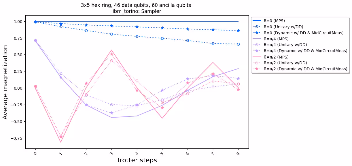
実験結果とシミュレーションを比較すると、動的回路の実装（星印付き点線）が標準的なユニタリ実装（丸印付き点線）よりも全体的に優れた性能を示していることがわかります。まとめとして、ハードウェアにネイティブではないトポロジーであるハニカム格子上のイジングスピンモデルのシミュレーションに対する解決策として動的回路を提示しました。動的回路による解決策は、SWAPゲートを使用する場合よりも短い2量子ビットゲート深さで、最近接でない量子ビット間のZZ相互作用を可能にします。その代償として、追加のアンシラ量子ビットと古典フィードフォワード演算が導入されます。

References

[1] Quantum computing with Qiskit, by Javadi-Abhari, A., Treinish, M., Krsulich, K., Wood, C.J., Lishman, J., Gacon, J., Martiel, S., Nation, P.D., Bishop, L.S., Cross, A.W. and Johnson, B.R., 2024. arXiv preprint arXiv:2405.08810 (2024)