ハミルトニアンシミュレーション回路のコンパイル手法
使用量の推定:IBM Heronプロセッサで1分未満(注意:これは推定値のみです。実際の実行時間は異なる場合があります。)
学習成果
このチュートリアルを通じて、以下を理解できるようになります:
- レイアウトおよびルーティング最適化のためのSABREを用いたQiskit Transpilerの使い方
- 高度な回路最適化のためのAI搭載トランスパイラの活用方法
- ハミルトニアンシミュレーション回路における
PauliEvolutionGate演算の合成のためのRustiqプラグインの使い方 - 2量子ビット深さ、総Gate数、実行時間を用いたコンパイル手法のベンチマーク・比較方法
前提条件
このチュートリアルを進める前に、以下のトピックに慣れておくことをお勧めします:
背景
量子Circuit のコンパイルは、高レベルの量子アルゴリズムをターゲットハードウェアの制約に準拠した物理回路に変換します。効果的なコンパイルにより、回路の深さとGate数を大幅に削減でき、これは近未来の量子デバイスにおける結果の品質に直接影響します。
このチュートリアルでは、PauliEvolutionGateを用いて構築されたハミルトニアンシミュレーション回路について、3つのコンパイル手法をベンチマークします。これらの回路はQubit間のペアワイズ相互作用(、、項など)をモデル化しており、量子化学、凝縮系物理学、材料科学において一般的に使用されます。
ベンチマーク回路はHamlibコレクションから取得し、Benchpressリポジトリを通じてアクセスします。Hamlibは代表的なハミルトニアンの標準化されたセットを提供しており、現実的なシミュレーションワークロードでコンパイル戦略を比較することができます。
コンパイル手法の概要
SABREを用いたQiskit Transpiler
Qiskit TranspilerはSABRE(SWAP-based BidiREctional heuristic search)アルゴリズムを使用して回路のレイアウトとルーティングを最適化します。SABREはハードウェアの接続性制約に準拠しながら、SWAPゲートとそれらが回路の深さに与える影響を最小化することに焦点を当てています。汎用的な手法であり、性能とコンパイル時間のバランスが優れています。詳細については[1]を参照してください。SABREの利点とパラメータ探索については、別のチュートリアルで詳しく扱っています。
AI搭載トランスパイラ
AI搭載トランスパイラは機械学習を使用して、回路構造とハードウェア制約のパターンを分析することで、最適なトランスパイル戦略を予測します。また、パウリネットワーク回路を強化学習ベースの合成アプローチで対象とするAIPauliNetworkSynthesisパスを適用することもできます。詳細については[2]および[3]を参照してください。
Rustiqプラグイン
Rustiqプラグインは、トロッター化ダイナミクスで一般的に使用されるパウリ回転を表すPauliEvolutionGate演算に特化した高度な合成技術を提供します。ハミルトニアンシミュレーションワークロードに対して低深さの回路分解を生成するように設計されています。詳細については[4]を参照してください。
主要なメトリクス
3つの手法を以下のメトリクスで比較します:
- 2量子ビット深さ:2量子ビットGateのみをカウントした回路の深さ。実際のハードウェアにおける忠実度のボトルネックとなることが多いです。
- 回路サイズ(総Gate数):トランスパイルされた回路の総Gate数。
- 実行時間:トランスパイルに要するウォールクロック時間。
要件
このチュートリアルを開始する前に、以下がインストールされていることを確認してください:
- Qiskit SDK v2.0以降、可視化サポート付き
- Qiskit Runtime v0.22以降(
pip install qiskit-ibm-runtime) - Qiskit Aer(
pip install qiskit-aer) - Qiskit IBM Transpiler(
pip install qiskit-ibm-transpiler) - Qiskit AI Transpiler ローカルモード(
pip install qiskit_ibm_ai_local_transpiler) - Networkx(
pip install networkx)
セットアップ
# Added by doQumentation — required packages for this notebook
!pip install -q matplotlib numpy qiskit qiskit-aer qiskit-ibm-runtime qiskit-ibm-transpiler requests scipy
from qiskit.circuit import QuantumCircuit
from qiskit_ibm_runtime import QiskitRuntimeService, SamplerV2
from qiskit.circuit.library import PauliEvolutionGate
from qiskit_ibm_transpiler import generate_ai_pass_manager
from qiskit.quantum_info import SparsePauliOp
from qiskit.transpiler.preset_passmanagers import generate_preset_pass_manager
from qiskit.transpiler.passes.synthesis.high_level_synthesis import HLSConfig
from qiskit_aer import AerSimulator
from qiskit_aer.noise import NoiseModel, depolarizing_error
from collections import Counter
from statistics import mean, stdev
from scipy.sparse import SparseEfficiencyWarning
import time
import warnings
import matplotlib.pyplot as plt
import matplotlib.ticker as ticker
import numpy as np
import json
import requests
import logging

# Suppress noisy loggers and warnings
logging.getLogger(
    "qiskit_ibm_transpiler.wrappers.ai_local_synthesis"
).setLevel(logging.ERROR)
warnings.filterwarnings("ignore", category=FutureWarning)
warnings.filterwarnings("ignore", category=SparseEfficiencyWarning)

seed = 42  # Seed for reproducibility
Backend への接続
小規模および大規模な例の両方に使用するBackend を選択します。Backend はTranspiler がターゲットとするカップリングマップと基底Gateを決定します。
# QiskitRuntimeService.save_account(channel="ibm_quantum_platform",
# token="<YOUR-API-KEY>", overwrite=True, set_as_default=True)
service = QiskitRuntimeService(channel="ibm_quantum_platform")
backend = service.least_busy(operational=True, simulator=False)
print(f"Using backend: {backend.name}")
Using backend: ibm_pittsburgh
パスマネージャーの定義
3つのコンパイル手法を設定します。
# SABRE pass manager (Qiskit default at optimization level 3)
pm_sabre = generate_preset_pass_manager(
    optimization_level=3, backend=backend, seed_transpiler=seed
)
# AI transpiler pass manager (local mode)
pm_ai = generate_ai_pass_manager(
    backend=backend, optimization_level=3, ai_optimization_level=3
)
Fetching 127 files: 0%| | 0/127 [00:00<?, ?it/s]
# Rustiq pass manager for PauliEvolutionGate synthesis
hls_config = HLSConfig(
    PauliEvolution=[
        (
            "rustiq",
            {
                "nshuffles": 400,
                "upto_phase": True,
                "fix_clifford": True,
                "preserve_order": False,
                "metric": "depth",
            },
        )
    ]
)
pm_rustiq = generate_preset_pass_manager(
    optimization_level=3,
    backend=backend,
    hls_config=hls_config,
    seed_transpiler=seed,
)
ヘルパー関数の定義
以下の関数は、指定されたパスマネージャーを使用してCircuit のリストをトランスパイルし、各回路の主要なメトリクス(2量子ビット深さ、回路サイズ、実行時間)を記録します。
def capture_transpilation_metrics(
    results, pass_manager, circuits, method_name
):
    """
    Transpile circuits and append one metrics record per circuit to
    ``results``.

    Args:
        results (list): List of dicts to append the metrics records to.
        pass_manager: Pass manager used for transpilation.
        circuits (list): List of quantum circuits to transpile.
        method_name (str): Name of the transpilation method.

    Returns:
        list: List of transpiled circuits.
    """
    transpiled_circuits = []

    for i, qc in enumerate(circuits):
        start_time = time.time()
        transpiled_qc = pass_manager.run(qc)
        end_time = time.time()

        # Decompose swaps for consistency across methods
        transpiled_qc = transpiled_qc.decompose(gates_to_decompose=["swap"])

        transpilation_time = end_time - start_time
        two_qubit_depth = transpiled_qc.depth(
            lambda x: x.operation.num_qubits == 2
        )
        circuit_size = transpiled_qc.size()

        results.append(
            {
                "method": method_name,
                "qc_name": qc.name,
                "qc_index": i,
                "num_qubits": qc.num_qubits,
                "two_qubit_depth": two_qubit_depth,
                "size": circuit_size,
                "runtime": transpilation_time,
            }
        )
        transpiled_circuits.append(transpiled_qc)
        print(
            f"[{method_name}] Circuit {i} ({qc.name}): "
            f"2Q depth={two_qubit_depth}, size={circuit_size}, "
            f"time={transpilation_time:.2f}s"
        )

    return transpiled_circuits
def _method_order(results):
    """Return the distinct method names in their first-seen order."""
    order = []
    for r in results:
        if r["method"] not in order:
            order.append(r["method"])
    return order

def print_summary_table(results):
    """
    Print the mean and standard deviation of each metric per compilation
    method, followed by the mean percent improvement relative to SABRE.
    """
    metrics = [
        ("two_qubit_depth", "2Q Depth"),
        ("size", "Gate Count"),
        ("runtime", "Runtime (s)"),
    ]
    methods = _method_order(results)
    by_method = {m: [r for r in results if r["method"] == m] for m in methods}
    sabre_by_index = {r["qc_index"]: r for r in by_method.get("SABRE", [])}

    col_w = 22
    name_w = max(len(m) for m in methods)
    header = f"{'Method':<{name_w}}" + "".join(
        f"  {label:>{col_w}}" for _, label in metrics
    )

    print("Mean +/- std per compilation method")
    print(header)
    print("-" * len(header))
    for method in methods:
        cells = []
        for key, _ in metrics:
            values = [r[key] for r in by_method[method]]
            std = stdev(values) if len(values) > 1 else 0.0
            cells.append(f"{mean(values):,.1f} +/- {std:,.1f}")
        print(
            f"{method:<{name_w}}" + "".join(f"  {c:>{col_w}}" for c in cells)
        )

    others = [m for m in methods if m != "SABRE"]
    if others and sabre_by_index:
        print()
        print("Mean % improvement vs SABRE (positive = better than SABRE)")
        print(header)
        print("-" * len(header))
        for method in others:
            cells = []
            for key, _ in metrics:
                pct = [
                    (sabre_by_index[r["qc_index"]][key] - r[key])
                    / sabre_by_index[r["qc_index"]][key]
                    * 100
                    for r in by_method[method]
                    if sabre_by_index.get(r["qc_index"])
                    and sabre_by_index[r["qc_index"]][key]
                ]
                if pct:
                    std = stdev(pct) if len(pct) > 1 else 0.0
                    cells.append(f"{mean(pct):+.1f}% +/- {std:.1f}%")
                else:
                    cells.append("n/a")
            print(
                f"{method:<{name_w}}"
                + "".join(f"  {c:>{col_w}}" for c in cells)
            )
def print_per_circuit_comparison(results, num_rows=5):
    """
    Print a per-metric comparison of the compilation methods for the
    first ``num_rows`` circuits (sorted by qubit count). The best
    (lowest) value for each metric is marked with an asterisk.
    """
    metrics = [
        ("two_qubit_depth", "2Q Depth"),
        ("size", "Gate Count"),
        ("runtime", "Runtime (s)"),
    ]
    methods = _method_order(results)

    by_index = {}
    for r in results:
        by_index.setdefault(r["qc_index"], {})[r["method"]] = r
    ordered = sorted(
        by_index.items(),
        key=lambda kv: (next(iter(kv[1].values()))["num_qubits"], kv[0]),
    )[:num_rows]

    for key, label in metrics:
        print(f"{label} (first {num_rows} circuits by qubit count); * = best")
        header = f"{'Idx':>3}  {'Circuit':<16} {'Q':>3}" + "".join(
            f"{m:>9}" for m in methods
        )
        print(header)
        print("-" * len(header))
        for idx, method_map in ordered:
            any_record = next(iter(method_map.values()))
            present = {
                m: method_map[m][key] for m in methods if m in method_map
            }
            best = min(present.values())
            line = (
                f"{idx:>3}  {any_record['qc_name'][:16]:<16} "
                f"{any_record['num_qubits']:>3}"
            )
            for m in methods:
                value = method_map[m][key]
                text = f"{value:.2f}" if key == "runtime" else f"{int(value)}"
                if value == best:
                    text += "*"
                line += f"{text:>9}"
            print(line)
        print()
HamlibからハミルトニアンCircuit をロードする
Benchpressリポジトリから代表的なハミルトニアンのセットをロードし、PauliEvolutionGate回路を構築します。Backend のQubit数を超えるCircuit は除外し、分解後のサイズが1,500Gateを超える回路も(トランスパイル時間を現実的な範囲に保つために)除外します。
# Obtain the Hamiltonian JSON from the benchpress repository
url = "https://raw.githubusercontent.com/Qiskit/benchpress/e7b29ef7be4cc0d70237b8fdc03edbd698908eff/benchpress/hamiltonian/hamlib/100_representative.json"
response = requests.get(url)
response.raise_for_status()
ham_records = json.loads(response.text)

# Remove circuits that are too large for the backend
ham_records = [
    h for h in ham_records if h["ham_qubits"] <= backend.num_qubits
]

# Build PauliEvolutionGate circuits
qc_ham_list = []
for h in ham_records:
    terms = h["ham_hamlib_hamiltonian_terms"]
    coeff = h["ham_hamlib_hamiltonian_coefficients"]
    num_qubits = h["ham_qubits"]
    name = h["ham_problem"]

    evo_gate = PauliEvolutionGate(SparsePauliOp(terms, coeff))
    qc = QuantumCircuit(num_qubits)
    qc.name = name
    qc.append(evo_gate, range(num_qubits))
    qc_ham_list.append(qc)

# Remove circuits whose decomposed size exceeds 1500 gates so that transpilation completes in a reasonable time frame
qc_ham_list = [qc for qc in qc_ham_list if qc.decompose().size() <= 1500]

print(f"Total Hamiltonian circuits loaded: {len(qc_ham_list)}")
print(
    f"Qubit range: {min(qc.num_qubits for qc in qc_ham_list)} to {max(qc.num_qubits for qc in qc_ham_list)}"
)
Total Hamiltonian circuits loaded: 42
Qubit range: 2 to 112
Circuit を小規模(20Qubit未満)と大規模(20Qubit以上)のグループに分割します。
qc_small = [qc for qc in qc_ham_list if qc.num_qubits < 20]
qc_large = [qc for qc in qc_ham_list if qc.num_qubits >= 20]

print(f"Small-scale circuits (<20 qubits): {len(qc_small)}")
print(f"Large-scale circuits (>=20 qubits): {len(qc_large)}")
Small-scale circuits (<20 qubits): 20
Large-scale circuits (>=20 qubits): 22
トランスパイル前に小規模なハミルトニアン回路の1つをプレビューします。
# We decompose the circuit here, otherwise it would just be a PauliEvolutionGate box,
# which isn't very informative to look at!
qc_small[0].decompose().draw("mpl", fold=-1)

小規模な例
このセクションでは、20Qubit未満のハミルトニアン回路に対して3つのコンパイル手法をベンチマークします。これらの回路は素早くトランスパイルでき、各手法が中程度の複雑さの回路をどのように処理するかを明確に確認できます。
ステップ1:古典的な入力を量子問題にマッピングする
各ハミルトニアンはPauliEvolutionGate回路としてエンコードされます。Circuit はセットアップセクションですでにHamlibベンチマークデータから構築されています。
ステップ2:量子ハードウェア実行のための問題の最適化
3つのパスマネージャーそれぞれを使用してすべての小規模Circuit をトランスパイルし、メトリクスを収集します。
results_small = []

tqc_sabre_small = capture_transpilation_metrics(
    results_small, pm_sabre, qc_small, "SABRE"
)
tqc_ai_small = capture_transpilation_metrics(
    results_small, pm_ai, qc_small, "AI"
)
tqc_rustiq_small = capture_transpilation_metrics(
    results_small, pm_rustiq, qc_small, "Rustiq"
)
[SABRE] Circuit 0 (all-vib-bh): 2Q depth=3, size=30, time=2.09s
[SABRE] Circuit 1 (all-vib-c2h): 2Q depth=18, size=111, time=0.01s
[SABRE] Circuit 2 (all-vib-o3): 2Q depth=6, size=58, time=0.00s
[SABRE] Circuit 3 (all-vib-c2h): 2Q depth=2, size=37, time=0.01s
[SABRE] Circuit 4 (graph-gnp_k-2): 2Q depth=24, size=126, time=0.01s
[SABRE] Circuit 5 (LiH): 2Q depth=66, size=285, time=0.01s
[SABRE] Circuit 6 (all-vib-fccf): 2Q depth=66, size=339, time=0.01s
[SABRE] Circuit 7 (all-vib-ch2): 2Q depth=88, size=413, time=0.01s
[SABRE] Circuit 8 (all-vib-f2): 2Q depth=180, size=1000, time=0.02s
[SABRE] Circuit 9 (all-vib-bhf2): 2Q depth=18, size=223, time=0.03s
[SABRE] Circuit 10 (graph-gnp_k-4): 2Q depth=122, size=675, time=0.02s
[SABRE] Circuit 11 (Be2): 2Q depth=343, size=1628, time=0.03s
[SABRE] Circuit 12 (all-vib-fccf): 2Q depth=14, size=134, time=0.00s
[SABRE] Circuit 13 (uf20-ham): 2Q depth=50, size=341, time=0.01s
[SABRE] Circuit 14 (TSP_Ncity-4): 2Q depth=118, size=615, time=0.01s
[SABRE] Circuit 15 (graph-complete_bipart): 2Q depth=232, size=1420, time=0.03s
[SABRE] Circuit 16 (all-vib-cyclo_propene): 2Q depth=18, size=354, time=0.93s
[SABRE] Circuit 17 (all-vib-hno): 2Q depth=6, size=174, time=0.14s
[SABRE] Circuit 18 (all-vib-fccf): 2Q depth=30, size=286, time=0.01s
[SABRE] Circuit 19 (tfim): 2Q depth=31, size=232, time=0.03s
[AI] Circuit 0 (all-vib-bh): 2Q depth=3, size=30, time=0.01s
Fetching 4 files: 0%| | 0/4 [00:00<?, ?it/s]
[AI] Circuit 1 (all-vib-c2h): 2Q depth=18, size=101, time=0.18s
[AI] Circuit 2 (all-vib-o3): 2Q depth=6, size=58, time=0.01s
[AI] Circuit 3 (all-vib-c2h): 2Q depth=2, size=37, time=0.01s
[AI] Circuit 4 (graph-gnp_k-2): 2Q depth=24, size=133, time=0.07s
[AI] Circuit 5 (LiH): 2Q depth=62, size=267, time=8.00s
[AI] Circuit 6 (all-vib-fccf): 2Q depth=65, size=300, time=0.18s
[AI] Circuit 7 (all-vib-ch2): 2Q depth=79, size=353, time=0.16s
[AI] Circuit 8 (all-vib-f2): 2Q depth=176, size=998, time=0.43s
[AI] Circuit 9 (all-vib-bhf2): 2Q depth=18, size=194, time=0.11s
[AI] Circuit 10 (graph-gnp_k-4): 2Q depth=114, size=668, time=0.18s
[AI] Circuit 11 (Be2): 2Q depth=292, size=1382, time=0.88s
[AI] Circuit 12 (all-vib-fccf): 2Q depth=14, size=134, time=0.01s
[AI] Circuit 13 (uf20-ham): 2Q depth=40, size=330, time=0.16s
[AI] Circuit 14 (TSP_Ncity-4): 2Q depth=96, size=600, time=0.29s
[AI] Circuit 15 (graph-complete_bipart): 2Q depth=231, size=1531, time=0.46s
[AI] Circuit 16 (all-vib-cyclo_propene): 2Q depth=18, size=309, time=0.25s
[AI] Circuit 17 (all-vib-hno): 2Q depth=10, size=198, time=0.15s
[AI] Circuit 18 (all-vib-fccf): 2Q depth=34, size=402, time=0.02s
[AI] Circuit 19 (tfim): 2Q depth=44, size=311, time=0.15s
[Rustiq] Circuit 0 (all-vib-bh): 2Q depth=3, size=30, time=0.01s
[Rustiq] Circuit 1 (all-vib-c2h): 2Q depth=13, size=69, time=0.00s
[Rustiq] Circuit 2 (all-vib-o3): 2Q depth=13, size=82, time=0.01s
[Rustiq] Circuit 3 (all-vib-c2h): 2Q depth=2, size=40, time=0.01s
[Rustiq] Circuit 4 (graph-gnp_k-2): 2Q depth=31, size=132, time=0.01s
[Rustiq] Circuit 5 (LiH): 2Q depth=59, size=285, time=0.01s
[Rustiq] Circuit 6 (all-vib-fccf): 2Q depth=34, size=193, time=0.00s
[Rustiq] Circuit 7 (all-vib-ch2): 2Q depth=49, size=302, time=0.01s
[Rustiq] Circuit 8 (all-vib-f2): 2Q depth=141, size=807, time=0.02s
[Rustiq] Circuit 9 (all-vib-bhf2): 2Q depth=13, size=146, time=0.02s
[Rustiq] Circuit 10 (graph-gnp_k-4): 2Q depth=129, size=683, time=0.02s
[Rustiq] Circuit 11 (Be2): 2Q depth=220, size=1101, time=0.02s
[Rustiq] Circuit 12 (all-vib-fccf): 2Q depth=53, size=333, time=0.01s
[Rustiq] Circuit 13 (uf20-ham): 2Q depth=63, size=425, time=0.01s
[Rustiq] Circuit 14 (TSP_Ncity-4): 2Q depth=123, size=767, time=0.02s
[Rustiq] Circuit 15 (graph-complete_bipart): 2Q depth=309, size=2107, time=0.05s
[Rustiq] Circuit 16 (all-vib-cyclo_propene): 2Q depth=16, size=283, time=0.32s
[Rustiq] Circuit 17 (all-vib-hno): 2Q depth=19, size=291, time=0.32s
[Rustiq] Circuit 18 (all-vib-fccf): 2Q depth=44, size=546, time=0.02s
[Rustiq] Circuit 19 (tfim): 2Q depth=24, size=416, time=0.01s
以下の表は、すべての小規模Circuit における各メトリクスの平均と標準偏差、およびSABREに対する改善率をまとめています。Circuit サイズが大きく異なるため、標準偏差は平均を解釈する上で重要なコンテキストを提供します。
print_summary_table(results_small)
Mean +/- std per compilation method
Method                2Q Depth              Gate Count             Runtime (s)
------------------------------------------------------------------------------
SABRE            71.8 +/- 89.6         424.1 +/- 446.0             0.2 +/- 0.5
AI               67.3 +/- 80.2         416.8 +/- 426.7             0.6 +/- 1.8
Rustiq           67.9 +/- 80.0         451.9 +/- 484.7             0.0 +/- 0.1

Mean % improvement vs SABRE (positive = better than SABRE)
Method                2Q Depth              Gate Count             Runtime (s)
------------------------------------------------------------------------------
AI             -2.1% +/- 19.8%         -0.6% +/- 14.7%   -5635.1% +/- 20725.2%
Rustiq        -25.3% +/- 85.4%        -16.3% +/- 50.4%         -7.0% +/- 60.6%
Circuit ごとの表は、個々の回路での各手法の比較を示しています。各メトリクスの最良値にはアスタリスクが付いています。最も単純な回路では、3つの手法が同じ結果に収束することが多いことに注目してください。
print_per_circuit_comparison(results_small, num_rows=8)
2Q Depth (first 8 circuits by qubit count); * = best
Idx  Circuit            Q    SABRE       AI   Rustiq
----------------------------------------------------
  0  all-vib-bh         2       3*       3*       3*
  1  all-vib-c2h        3       18       18      13*
  2  all-vib-o3         4       6*       6*       13
  3  all-vib-c2h        4       2*       2*       2*
  4  graph-gnp_k-2      4      24*      24*       31
  5  LiH                4       66       62      59*
  6  all-vib-fccf       4       66       65      34*
  7  all-vib-ch2        4       88       79      49*

Gate Count (first 8 circuits by qubit count); * = best
Idx  Circuit            Q    SABRE       AI   Rustiq
----------------------------------------------------
  0  all-vib-bh         2      30*      30*      30*
  1  all-vib-c2h        3      111      101      69*
  2  all-vib-o3         4      58*      58*       82
  3  all-vib-c2h        4      37*      37*       40
  4  graph-gnp_k-2      4     126*      133      132
  5  LiH                4      285     267*      285
  6  all-vib-fccf       4      339      300     193*
  7  all-vib-ch2        4      413      353     302*

Runtime (s) (first 8 circuits by qubit count); * = best
Idx  Circuit            Q    SABRE       AI   Rustiq
----------------------------------------------------
  0  all-vib-bh         2     2.09     0.01    0.01*
  1  all-vib-c2h        3     0.01     0.18    0.00*
  2  all-vib-o3         4    0.00*     0.01     0.01
  3  all-vib-c2h        4     0.01     0.01    0.01*
  4  graph-gnp_k-2      4    0.01*     0.07     0.01
  5  LiH                4    0.01*     8.00     0.01
  6  all-vib-fccf       4     0.01     0.18    0.00*
  7  all-vib-ch2        4     0.01     0.16    0.01*
結果の可視化
以下のプロットは、各メトリクスにおける3つの手法の回路ごとの比較を示しています。Circuit はQubit数でソートされ、x軸にはインデックスでラベル付けされています(同じQubit数の回路が複数存在する場合があるため)。
def plot_transpilation_comparison(results, title_prefix):
    """
    Create a three-panel figure comparing compilation methods on
    two-qubit depth, circuit size, and runtime.

    Circuits are sorted by qubit count and plotted by circuit index.
    """
    methods = _method_order(results)
    palette = {"SABRE": "#1f77b4", "AI": "#ff7f0e", "Rustiq": "#2ca02c"}
    markers = {"SABRE": "o", "AI": "^", "Rustiq": "s"}

    # Order circuits by qubit count (then index) and map to plot positions
    ref = sorted(
        [r for r in results if r["method"] == methods[0]],
        key=lambda r: (r["num_qubits"], r["qc_index"]),
    )
    pos_map = {r["qc_index"]: pos for pos, r in enumerate(ref)}
    tick_positions = [pos_map[r["qc_index"]] for r in ref]
    tick_labels = [
        f"{pos_map[r['qc_index']]} ({r['num_qubits']}q)" for r in ref
    ]

    metrics = [
        ("two_qubit_depth", "Two-Qubit Depth"),
        ("size", "Total Gate Count (Circuit Size)"),
        ("runtime", "Transpilation Runtime (s)"),
    ]

    fig, axes = plt.subplots(1, 3, figsize=(20, 5.5))
    fig.suptitle(title_prefix, fontsize=15, fontweight="bold", y=1.02)

    for ax, (metric, ylabel) in zip(axes, metrics):
        for method in methods:
            subset = sorted(
                [r for r in results if r["method"] == method],
                key=lambda r: pos_map[r["qc_index"]],
            )
            ax.plot(
                [pos_map[r["qc_index"]] for r in subset],
                [r[metric] for r in subset],
                marker=markers.get(method, "o"),
                label=method,
                color=palette.get(method, None),
                linewidth=1.5,
                markersize=6,
                alpha=0.85,
            )
        ax.set_xlabel("Circuit Index (num qubits)", fontsize=11)
        ax.set_ylabel(ylabel, fontsize=11)
        ax.legend(frameon=True, fontsize=9)
        ax.grid(True, linestyle="--", alpha=0.4)
        step = max(1, len(tick_positions) // 15)
        ax.set_xticks(tick_positions[::step])
        ax.set_xticklabels(
            [tick_labels[i] for i in range(0, len(tick_labels), step)],
            fontsize=7,
            rotation=45,
            ha="right",
        )

    plt.tight_layout()
    plt.show()
def plot_pct_improvement_vs_sabre(results, title_prefix):
    """
    Plot the per-circuit percent improvement of each non-SABRE method
    relative to SABRE, for each metric. A positive value means the
    method improved on SABRE; negative means SABRE was better.
    """
    metrics = [
        ("two_qubit_depth", "2Q Depth"),
        ("size", "Gate Count"),
        ("runtime", "Runtime"),
    ]
    palette = {"AI": "#ff7f0e", "Rustiq": "#2ca02c"}
    markers = {"AI": "^", "Rustiq": "s"}

    methods = _method_order(results)
    sabre = sorted(
        [r for r in results if r["method"] == "SABRE"],
        key=lambda r: (r["num_qubits"], r["qc_index"]),
    )
    other_methods = [m for m in methods if m != "SABRE"]

    tick_positions = list(range(len(sabre)))
    tick_labels = [
        f"{i} ({sabre[i]['num_qubits']}q)" for i in range(len(sabre))
    ]

    fig, axes = plt.subplots(1, 3, figsize=(20, 5.5))
    fig.suptitle(
        f"{title_prefix}: % Improvement over SABRE",
        fontsize=15,
        fontweight="bold",
        y=1.02,
    )

    for ax, (metric, label) in zip(axes, metrics):
        ax.axhline(0, color="#1f77b4", linewidth=2, label="SABRE (baseline)")
        for method in other_methods:
            data = sorted(
                [r for r in results if r["method"] == method],
                key=lambda r: (r["num_qubits"], r["qc_index"]),
            )
            pct = [
                (sabre[i][metric] - data[i][metric]) / sabre[i][metric] * 100
                for i in range(len(sabre))
            ]
            ax.plot(
                tick_positions,
                pct,
                marker=markers.get(method, "o"),
                label=method,
                color=palette.get(method, None),
                linewidth=1.5,
                markersize=6,
                alpha=0.85,
            )
        ax.set_xlabel("Circuit Index (num qubits)", fontsize=11)
        ax.set_ylabel(f"% Improvement ({label})", fontsize=11)
        ax.legend(frameon=True, fontsize=9)
        ax.grid(True, linestyle="--", alpha=0.4)
        step = max(1, len(tick_positions) // 15)
        ax.set_xticks(tick_positions[::step])
        ax.set_xticklabels(
            [tick_labels[i] for i in range(0, len(tick_labels), step)],
            fontsize=7,
            rotation=45,
            ha="right",
        )
        ylims = ax.get_ylim()
        ax.axhspan(0, max(ylims[1], 1), alpha=0.04, color="green")
        ax.axhspan(min(ylims[0], -1), 0, alpha=0.04, color="red")

    plt.tight_layout()
    plt.show()
plot_transpilation_comparison(
    results_small,
    "Small-Scale Hamiltonian Circuits: Compilation Comparison",
)
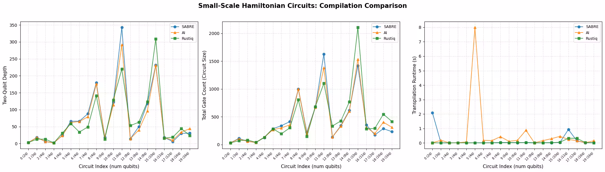
plot_pct_improvement_vs_sabre(
    results_small,
    "Small-Scale Hamiltonian Circuits",
)
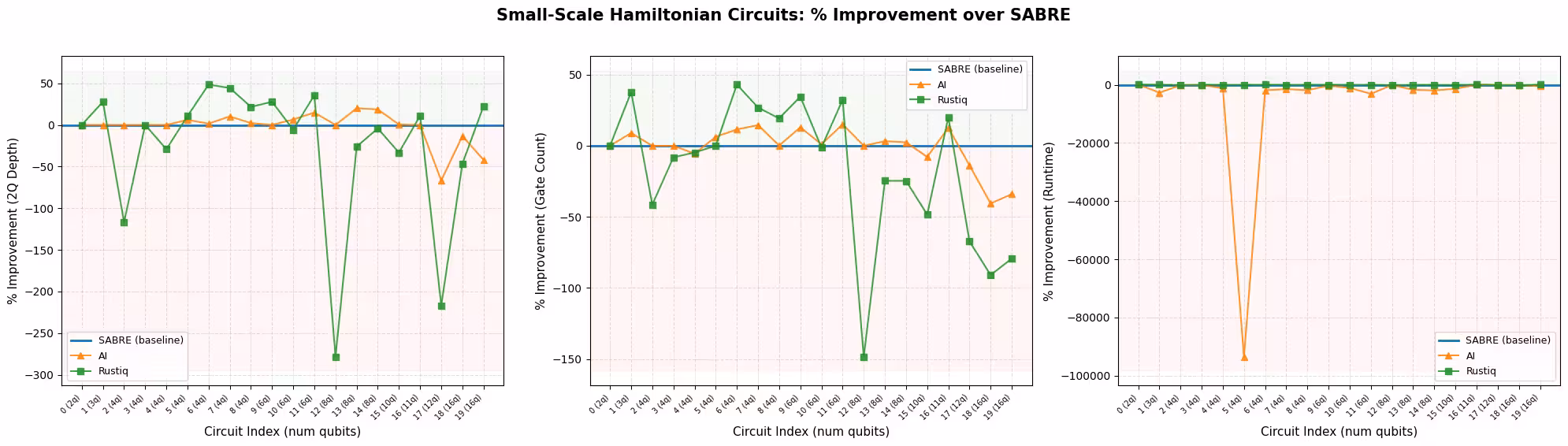
このスケールでは、3つのパスマネージャーはいずれも良好に動作し、平均的な結果は互いに近接しています。これは主に、小規模回路には最適化の余地が限られており、手法が同様の解に収束する傾向があるためです。
この例では、Rustiqは2量子ビット深さとGate数の両方で最も大きな外れ値を持つ、最も変動の大きい結果を生成しています。この変動性は時に他の2手法より劣ることを意味しますが、Rustiqが他の2つよりも優れた解を見つけることもあります。AIトランスパイラはSABREとRustiqに対してより安定した結果を示し、大部分の回路でほぼ追随し、外れ値も少ないです。
実行時間については、SABREとRustiqはともに高速ですが、AI搭載トランスパイラは特定の回路で著しく遅くなります。
メトリクスごとに最良の手法
以下のグラフは、各メトリクスで最良値(最小値)を達成した手法の割合を示しています。タイも可能です:単純な回路では、複数の手法が同じ最適な2量子ビット深さやGate数に到達できます。タイが発生した場合、すべてのタイした手法がクレジットを受けるため、あるメトリクスのパーセンテージの合計が100%を超える場合があります。
def plot_best_method_bars(results, metrics_list=None):
    """
    Plot a grouped bar chart showing the percentage of circuits
    where each method achieved the best (lowest) value for each metric.

    Ties are counted for all tied methods, so percentages per metric
    can sum to more than 100%.
    """
    if metrics_list is None:
        metrics_list = ["two_qubit_depth", "size", "runtime"]

    labels = {
        "two_qubit_depth": "2Q Depth",
        "size": "Gate Count",
        "runtime": "Runtime",
    }
    methods = _method_order(results)
    palette = {"SABRE": "#1f77b4", "AI": "#ff7f0e", "Rustiq": "#2ca02c"}

    by_index = {}
    for r in results:
        by_index.setdefault(r["qc_index"], []).append(r)
    n_circuits = len(by_index)

    win_data = {m: [] for m in methods}
    tie_counts = []
    metric_labels = []

    for metric in metrics_list:
        metric_labels.append(
            labels.get(metric, metric.replace("_", " ").title())
        )
        counts = Counter()
        ties = 0
        for group in by_index.values():
            min_val = min(r[metric] for r in group)
            best = [r["method"] for r in group if r[metric] == min_val]
            if len(best) > 1:
                ties += 1
            counts.update(best)
        tie_counts.append(ties)
        for m in methods:
            win_data[m].append(counts.get(m, 0) / n_circuits * 100)

    x = np.arange(len(metric_labels))
    width = 0.22
    fig, ax = plt.subplots(figsize=(8, 5))

    for i, method in enumerate(methods):
        bars = ax.bar(
            x + i * width,
            win_data[method],
            width,
            label=method,
            color=palette.get(method, None),
            edgecolor="black",
            linewidth=0.5,
        )
        for bar in bars:
            height = bar.get_height()
            if height > 0:
                ax.text(
                    bar.get_x() + bar.get_width() / 2,
                    height + 1.5,
                    f"{height:.0f}%",
                    ha="center",
                    va="bottom",
                    fontsize=9,
                )

    # Annotate tie counts below each metric label
    for j, ties in enumerate(tie_counts):
        if ties > 0:
            ax.text(
                x[j] + width,
                -8,
                f"({ties} tie{'s' if ties != 1 else ''})",
                ha="center",
                va="top",
                fontsize=8,
                color="gray",
            )

    ax.set_xticks(x + width)
    ax.set_xticklabels(metric_labels, fontsize=11)
    ax.set_ylabel("Circuits with best value (%)", fontsize=11)
    ax.set_title(
        "Best-Performing Method by Metric (ties counted for all tied methods)",
        fontsize=12,
        fontweight="bold",
    )
    ax.legend(frameon=True, fontsize=10)
    ax.set_ylim(-12, 120)
    ax.yaxis.set_major_formatter(ticker.PercentFormatter())
    ax.grid(axis="y", linestyle="--", alpha=0.4)

    plt.tight_layout()
    plt.show()
plot_best_method_bars(results_small)

この例では、3つの手法は小規模回路で非常に類似した性能を示しています。2量子ビット深さとGate数において、各手法が最良となる回路の割合は近接しており(おおよそ35〜55%)、最も単純な回路では複数の手法が同じ最適解を見つけるためタイとなる回路も多くあります。最も明確な違いは実行時間です:SABREとRustiqはそれぞれ約半数の回路で最速を達成していますが、AI搭載トランスパイラが最速となることはほとんどありません。3つのメトリクスすべてを総合的に考慮すると、Rustiqにわずかな全体的優位性があります 2量子ビット深さで最も頻繁に勝者となり、Gate数と実行時間でも競争力を維持しています。
ステップ3:Qiskitプリミティブを使用した実行
ノイズ下でのトランスパイル品質が実行にどう影響するかを評価するために、ミラー回路技術を使用します。各トランスパイル済みCircuit について、その逆回路を付加し、組み合わせた回路が理論的に恒等演算となるようにします。状態から始めた場合、完璧な(ノイズなし)実行では全ゼロのビット列が確率1で返されます。
実際には、回路全体でGateエラーが蓄積するため、を回復する確率が低下します。より浅い回路とより少ないGateを生成するコンパイル手法は、蓄積するノイズが少なくなります。
ミラー回路アプローチは魅力的なほどシンプルで、任意の回路サイズにスケールします。期待される出力は常にであり、理想状態の古典的シミュレーションは不要だからです。ただし、以下の注意点があります:ミラー回路は実際の回路のプロキシです(回路そのものではありません)、Gate数が2倍になります(ノイズの影響を誇張します)、ノイズがミラー境界を対称的にキャンセルする場合、特定のエラーを過小評価する可能性があります。
小規模セットから回路インデックス6を選択し、単純な脱分極ノイズモデルを使用したAerシミュレータでミラー回路を実行します。
# Select circuit index 6 from the small-scale transpiled circuits
test_idx = 6
test_circuit = qc_small[test_idx]
print(f"Test circuit: {test_circuit.name}, {test_circuit.num_qubits} qubits")

# Get the transpiled versions
tqc_methods_small = {
    "SABRE": tqc_sabre_small[test_idx],
    "AI": tqc_ai_small[test_idx],
    "Rustiq": tqc_rustiq_small[test_idx],
}

# Show transpilation metrics for this circuit
print(f"\nTranspilation metrics for circuit index {test_idx}:")
for method, tqc in tqc_methods_small.items():
    depth_2q = tqc.depth(lambda x: x.operation.num_qubits == 2)
    size = tqc.size()
    print(f"  {method:8s}  2Q depth={depth_2q:5d}  size={size:6d}")
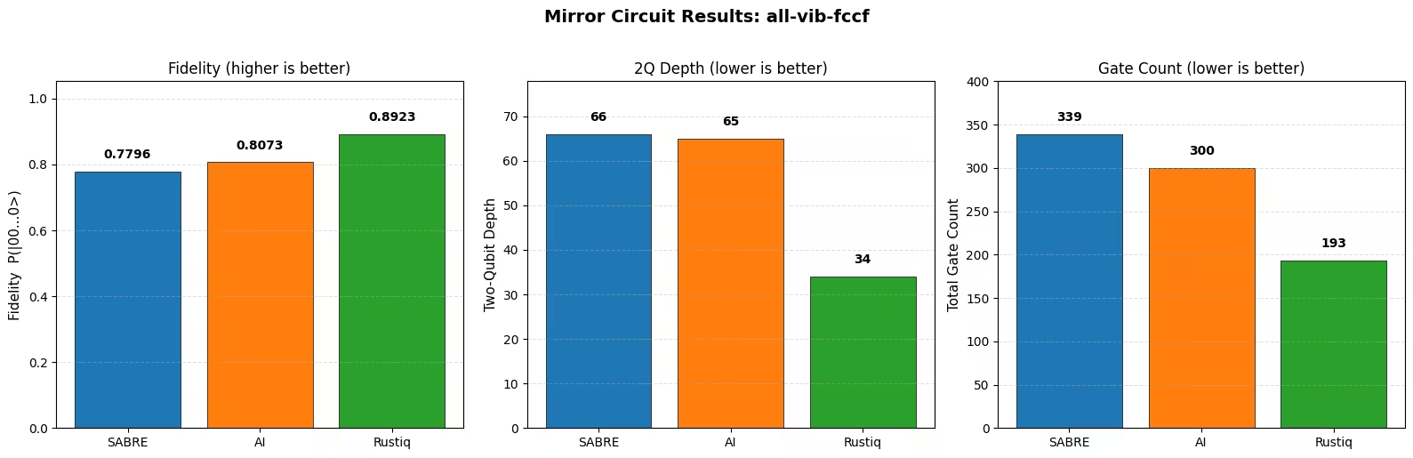
Test circuit: all-vib-fccf, 4 qubits

Transpilation metrics for circuit index 6:
  SABRE     2Q depth=   66  size=   339
  AI        2Q depth=   65  size=   300
  Rustiq    2Q depth=   34  size=   193
ミラー回路(を付加)を構築し、連続したQubitインデックスに再マッピングしてシミュレータがアクティブなQubitのみを処理するようにし、ノイズを含むAerシミュレータで実行します。
def remap_to_contiguous(tqc):
    """Remap a transpiled circuit to use contiguous qubit indices.

    Transpiled circuits target specific physical qubits (e.g., qubit 45, 67)
    on a large backend. This remaps them to 0, 1, 2, ... so Aer only
    simulates the active qubits.
    """
    active = sorted(
        {tqc.find_bit(q).index for inst in tqc.data for q in inst.qubits}
    )
    qubit_map = {old: new for new, old in enumerate(active)}
    new_qc = QuantumCircuit(len(active))
    for inst in tqc.data:
        old_indices = [tqc.find_bit(q).index for q in inst.qubits]
        new_qc.append(inst.operation, [qubit_map[i] for i in old_indices])
    return new_qc

def build_mirror_circuit(tqc):
    """Build a mirror circuit: U followed by U-dagger, with measurements.

    The combined circuit U-dagger @ U should be the identity, so measuring
    all zeros indicates a noise-free execution.
    """
    tqc_compact = remap_to_contiguous(tqc)
    mirror = tqc_compact.compose(tqc_compact.inverse())
    mirror.measure_all()
    return mirror

# Build a simple depolarizing noise model
noise_model = NoiseModel()
noise_model.add_all_qubit_quantum_error(
    depolarizing_error(0.001, 1),
    ["sx", "x", "rz"],  # ~0.1% per 1Q gate
)
noise_model.add_all_qubit_quantum_error(
    depolarizing_error(0.01, 2),
    ["cx", "ecr"],  # ~1% per 2Q gate
)

aer_sim = AerSimulator(noise_model=noise_model)

shots = 10000
fidelities = {}

for method, tqc in tqc_methods_small.items():
    mirror = build_mirror_circuit(tqc)

    sampler = SamplerV2(mode=aer_sim)
    job = sampler.run([mirror], shots=shots)
    result = job.result()
    counts = result[0].data.meas.get_counts()

    # Fidelity = fraction of all-zeros (error-free) outcomes
    n_qubits = mirror.num_qubits - mirror.num_clbits  # active qubits
    all_zeros = "0" * mirror.num_qubits
    fidelity = counts.get(all_zeros, 0) / shots
    fidelities[method] = fidelity
    print(
        f"{method:8s}  P(|00...0>) = {fidelity:.4f}  ({counts.get(all_zeros, 0)}/{shots})"
    )
SABRE     P(|00...0>) = 0.7796  (7796/10000)
AI        P(|00...0>) = 0.8073  (8073/10000)
Rustiq    P(|00...0>) = 0.8923  (8923/10000)
def plot_mirror_results(tqc_methods, fidelities, circuit_name):
    """
    Plot a three-panel comparison: fidelity, 2Q depth,
    and gate count for each compilation method.
    """
    methods = list(tqc_methods.keys())
    palette = {"SABRE": "#1f77b4", "AI": "#ff7f0e", "Rustiq": "#2ca02c"}
    colors = [palette.get(m, "gray") for m in methods]

    fidelity_vals = [fidelities[m] for m in methods]
    depth_vals = [
        tqc_methods[m].depth(lambda x: x.operation.num_qubits == 2)
        for m in methods
    ]
    size_vals = [tqc_methods[m].size() for m in methods]

    fig, axes = plt.subplots(1, 3, figsize=(16, 5))
    fig.suptitle(
        f"Mirror Circuit Results: {circuit_name}",
        fontsize=14,
        fontweight="bold",
        y=1.02,
    )

    def _annotate_bars(ax, bars, values, fmt="{}"):
        ymax = ax.get_ylim()[1]
        for bar, val in zip(bars, values):
            label = fmt.format(val)
            y = val + ymax * 0.03
            ax.text(
                bar.get_x() + bar.get_width() / 2,
                y,
                label,
                ha="center",
                va="bottom",
                fontsize=10,
                fontweight="bold",
            )

    # Panel 1: Survival Probability
    bars = axes[0].bar(
        methods, fidelity_vals, color=colors, edgecolor="black", linewidth=0.5
    )
    axes[0].set_ylabel("Fidelity  P(|00...0>)", fontsize=11)
    axes[0].set_title("Fidelity (higher is better)", fontsize=12)
    axes[0].set_ylim(
        0, max(fidelity_vals) * 1.18 if max(fidelity_vals) > 0 else 1.0
    )
    axes[0].grid(axis="y", linestyle="--", alpha=0.4)
    _annotate_bars(axes[0], bars, fidelity_vals, fmt="{:.4f}")

    # Panel 2: Two-Qubit Depth
    bars = axes[1].bar(
        methods, depth_vals, color=colors, edgecolor="black", linewidth=0.5
    )
    axes[1].set_ylabel("Two-Qubit Depth", fontsize=11)
    axes[1].set_title("2Q Depth (lower is better)", fontsize=12)
    axes[1].set_ylim(0, max(depth_vals) * 1.18)
    axes[1].grid(axis="y", linestyle="--", alpha=0.4)
    _annotate_bars(axes[1], bars, depth_vals)

    # Panel 3: Gate Count
    bars = axes[2].bar(
        methods, size_vals, color=colors, edgecolor="black", linewidth=0.5
    )
    axes[2].set_ylabel("Total Gate Count", fontsize=11)
    axes[2].set_title("Gate Count (lower is better)", fontsize=12)
    axes[2].set_ylim(0, max(size_vals) * 1.18)
    axes[2].grid(axis="y", linestyle="--", alpha=0.4)
    _annotate_bars(axes[2], bars, size_vals)

    plt.tight_layout()
    plt.show()

plot_mirror_results(tqc_methods_small, fidelities, test_circuit.name)
観察結果
2量子ビット深さが最も低く、Gate数が最も少ない手法が最も高い忠実度を達成しており、これは浅い回路ほど蓄積するノイズが少ないという期待と一致しています。深さとGate数のわずかな差でも、脱分極ノイズモデル下では忠実度の測定可能な差につながります。
これらの結果は単一の回路に対するものであることに留意してください。手法の相対的な順位は、ハミルトニアンの構造によって回路ごとに変わる可能性があります。
大規模なハードウェアの例
このセクションでは、20Qubit以上のハミルトニアン回路に対して同じ3つのコンパイル手法をベンチマークします。これらの回路は実際のハミルトニアンシミュレーションワークロードをより代表しており、各手法が回路品質とコンパイル時間においてどのようにスケールするかをテストします。
ステップ1〜4の統合
ワークフローは小規模な例と同じ構造に従います。各手法を使用してすべての大規模Circuit をトランスパイルし、メトリクスを収集し、ミラー回路を実際の量子ハードウェアに送信します。
results_large = []

tqc_sabre_large = capture_transpilation_metrics(
    results_large, pm_sabre, qc_large, "SABRE"
)
tqc_ai_large = capture_transpilation_metrics(
    results_large, pm_ai, qc_large, "AI"
)
tqc_rustiq_large = capture_transpilation_metrics(
    results_large, pm_rustiq, qc_large, "Rustiq"
)
[SABRE] Circuit 0 (all-vib-hc3h2cn): 2Q depth=2, size=258, time=0.16s
[SABRE] Circuit 1 (ham-graph-gnp_k-5): 2Q depth=345, size=4036, time=0.08s
[SABRE] Circuit 2 (TSP_Ncity-5): 2Q depth=187, size=2045, time=0.04s
[SABRE] Circuit 3 (tfim): 2Q depth=100, size=489, time=0.21s
[SABRE] Circuit 4 (all-vib-h2co): 2Q depth=30, size=570, time=0.18s
[SABRE] Circuit 5 (uuf100-ham): 2Q depth=414, size=4779, time=0.09s
[SABRE] Circuit 6 (uuf100-ham): 2Q depth=523, size=5667, time=0.11s
[SABRE] Circuit 7 (graph-gnp_k-4): 2Q depth=3028, size=24885, time=0.39s
[SABRE] Circuit 8 (uf100-ham): 2Q depth=700, size=8271, time=0.15s
[SABRE] Circuit 9 (uf100-ham): 2Q depth=698, size=8957, time=0.15s
[SABRE] Circuit 10 (TSP_Ncity-7): 2Q depth=432, size=6353, time=0.12s
[SABRE] Circuit 11 (all-vib-cyclo_propene): 2Q depth=30, size=1144, time=0.20s
[SABRE] Circuit 12 (TSP_Ncity-8): 2Q depth=704, size=10287, time=0.18s
[SABRE] Circuit 13 (uf100-ham): 2Q depth=2454, size=30195, time=0.46s
[SABRE] Circuit 14 (tfim): 2Q depth=245, size=3670, time=0.08s
[SABRE] Circuit 15 (flat100-ham): 2Q depth=154, size=3836, time=0.12s
[SABRE] Circuit 16 (graph-regular_reg-4): 2Q depth=863, size=14063, time=0.22s
[SABRE] Circuit 17 (tfim): 2Q depth=581, size=8810, time=0.15s
[SABRE] Circuit 18 (FH_D-1): 2Q depth=1704, size=9528, time=0.35s
[SABRE] Circuit 19 (TSP_Ncity-10): 2Q depth=1091, size=22041, time=0.38s
[SABRE] Circuit 20 (TSP_Ncity-10): 2Q depth=1091, size=22005, time=0.38s
[SABRE] Circuit 21 (ham-unary-color02-queen13_13_k-4): 2Q depth=224, size=8321, time=0.17s
[AI] Circuit 0 (all-vib-hc3h2cn): 2Q depth=2, size=258, time=0.17s
[AI] Circuit 1 (ham-graph-gnp_k-5): 2Q depth=323, size=4418, time=3.13s
[AI] Circuit 2 (TSP_Ncity-5): 2Q depth=161, size=2229, time=1.47s
[AI] Circuit 3 (tfim): 2Q depth=20, size=402, time=0.34s
[AI] Circuit 4 (all-vib-h2co): 2Q depth=38, size=661, time=0.19s
[AI] Circuit 5 (uuf100-ham): 2Q depth=391, size=5130, time=3.27s
[AI] Circuit 6 (uuf100-ham): 2Q depth=463, size=6095, time=4.23s
[AI] Circuit 7 (graph-gnp_k-4): 2Q depth=3207, size=25641, time=15.15s
[AI] Circuit 8 (uf100-ham): 2Q depth=637, size=8267, time=5.87s
[AI] Circuit 9 (uf100-ham): 2Q depth=632, size=9330, time=7.29s
[AI] Circuit 10 (TSP_Ncity-7): 2Q depth=452, size=7418, time=6.02s
[AI] Circuit 11 (all-vib-cyclo_propene): 2Q depth=38, size=1323, time=0.27s
[AI] Circuit 12 (TSP_Ncity-8): 2Q depth=609, size=11131, time=10.07s
[AI] Circuit 13 (uf100-ham): 2Q depth=2251, size=31128, time=38.77s
[AI] Circuit 14 (tfim): 2Q depth=165, size=3460, time=1.64s
[AI] Circuit 15 (flat100-ham): 2Q depth=91, size=3497, time=2.49s
[AI] Circuit 16 (graph-regular_reg-4): 2Q depth=664, size=15256, time=12.35s
[AI] Circuit 17 (tfim): 2Q depth=583, size=9157, time=6.28s
[AI] Circuit 18 (FH_D-1): 2Q depth=1193, size=7754, time=4.54s
[AI] Circuit 19 (TSP_Ncity-10): 2Q depth=1134, size=22577, time=25.64s
[AI] Circuit 20 (TSP_Ncity-10): 2Q depth=1172, size=23851, time=28.97s
[AI] Circuit 21 (ham-unary-color02-queen13_13_k-4): 2Q depth=219, size=8600, time=8.85s
[Rustiq] Circuit 0 (all-vib-hc3h2cn): 2Q depth=2, size=257, time=0.16s
[Rustiq] Circuit 1 (ham-graph-gnp_k-5): 2Q depth=640, size=5831, time=0.13s
[Rustiq] Circuit 2 (TSP_Ncity-5): 2Q depth=408, size=3985, time=0.08s
[Rustiq] Circuit 3 (tfim): 2Q depth=31, size=688, time=0.07s
[Rustiq] Circuit 4 (all-vib-h2co): 2Q depth=65, size=1058, time=2.91s
[Rustiq] Circuit 5 (uuf100-ham): 2Q depth=633, size=6757, time=0.14s
[Rustiq] Circuit 6 (uuf100-ham): 2Q depth=795, size=8495, time=0.17s
[Rustiq] Circuit 7 (graph-gnp_k-4): 2Q depth=13768, size=139793, time=2.92s
[Rustiq] Circuit 8 (uf100-ham): 2Q depth=1099, size=11878, time=0.25s
[Rustiq] Circuit 9 (uf100-ham): 2Q depth=911, size=11111, time=0.22s
[Rustiq] Circuit 10 (TSP_Ncity-7): 2Q depth=1183, size=13197, time=0.27s
[Rustiq] Circuit 11 (all-vib-cyclo_propene): 2Q depth=67, size=2491, time=13.56s
[Rustiq] Circuit 12 (TSP_Ncity-8): 2Q depth=1615, size=21358, time=0.48s
[Rustiq] Circuit 13 (uf100-ham): 2Q depth=2920, size=40465, time=0.91s
[Rustiq] Circuit 14 (tfim): 2Q depth=489, size=6552, time=0.15s
[Rustiq] Circuit 15 (flat100-ham): 2Q depth=378, size=5906, time=0.14s
[Rustiq] Circuit 16 (graph-regular_reg-4): 2Q depth=12163, size=168679, time=2.94s
[Rustiq] Circuit 17 (tfim): 2Q depth=1208, size=17042, time=0.36s
[Rustiq] Circuit 18 (FH_D-1): 2Q depth=1061, size=24000, time=0.47s
[Rustiq] Circuit 19 (TSP_Ncity-10): 2Q depth=2565, size=41340, time=1.38s
[Rustiq] Circuit 20 (TSP_Ncity-10): 2Q depth=2565, size=41275, time=1.38s
[Rustiq] Circuit 21 (ham-unary-color02-queen13_13_k-4): 2Q depth=808, size=17548, time=0.42s
print_summary_table(results_large)
Mean +/- std per compilation method
Method                2Q Depth              Gate Count             Runtime (s)
------------------------------------------------------------------------------
SABRE          709.1 +/- 783.8     9,100.5 +/- 8,493.1             0.2 +/- 0.1
AI             656.6 +/- 777.5     9,435.6 +/- 8,853.0            8.5 +/- 10.2
Rustiq     2,062.5 +/- 3,631.1   26,804.8 +/- 43,403.1             1.3 +/- 2.9

Mean % improvement vs SABRE (positive = better than SABRE)
Method                2Q Depth              Gate Count             Runtime (s)
------------------------------------------------------------------------------
AI             +9.6% +/- 22.8%          -3.4% +/- 9.4%    -3620.0% +/- 2405.5%
Rustiq      -154.5% +/- 273.9%      -137.1% +/- 233.2%     -527.0% +/- 1405.5%
print_per_circuit_comparison(results_large, num_rows=8)
2Q Depth (first 8 circuits by qubit count); * = best
Idx  Circuit            Q    SABRE       AI   Rustiq
----------------------------------------------------
  0  all-vib-hc3h2cn   24       2*       2*       2*
  1  ham-graph-gnp_k-  24      345     323*      640
  2  TSP_Ncity-5       25      187     161*      408
  3  tfim              26      100      20*       31
  4  all-vib-h2co      32      30*       38       65
  5  uuf100-ham        40      414     391*      633
  6  uuf100-ham        40      523     463*      795
  7  graph-gnp_k-4     40    3028*     3207    13768

Gate Count (first 8 circuits by qubit count); * = best
Idx  Circuit            Q    SABRE       AI   Rustiq
----------------------------------------------------
  0  all-vib-hc3h2cn   24      258      258     257*
  1  ham-graph-gnp_k-  24    4036*     4418     5831
  2  TSP_Ncity-5       25    2045*     2229     3985
  3  tfim              26      489     402*      688
  4  all-vib-h2co      32     570*      661     1058
  5  uuf100-ham        40    4779*     5130     6757
  6  uuf100-ham        40    5667*     6095     8495
  7  graph-gnp_k-4     40   24885*    25641   139793

Runtime (s) (first 8 circuits by qubit count); * = best
Idx  Circuit            Q    SABRE       AI   Rustiq
----------------------------------------------------
  0  all-vib-hc3h2cn   24     0.16     0.17    0.16*
  1  ham-graph-gnp_k-  24    0.08*     3.13     0.13
  2  TSP_Ncity-5       25    0.04*     1.47     0.08
  3  tfim              26     0.21     0.34    0.07*
  4  all-vib-h2co      32    0.18*     0.19     2.91
  5  uuf100-ham        40    0.09*     3.27     0.14
  6  uuf100-ham        40    0.11*     4.23     0.17
  7  graph-gnp_k-4     40    0.39*    15.15     2.92
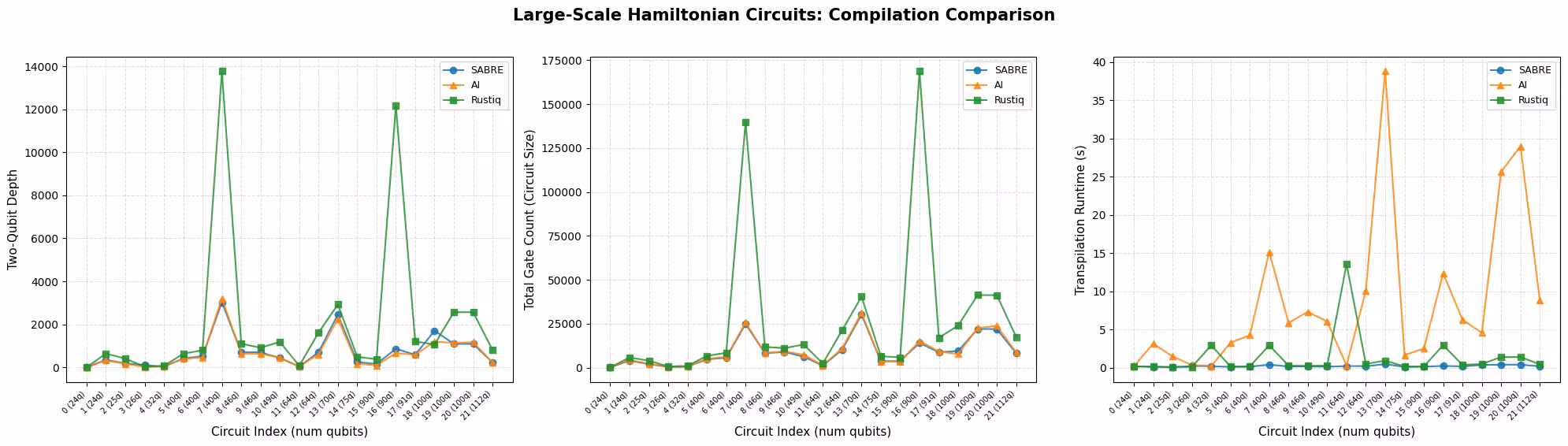
plot_transpilation_comparison(
    results_large,
    "Large-Scale Hamiltonian Circuits: Compilation Comparison",
)
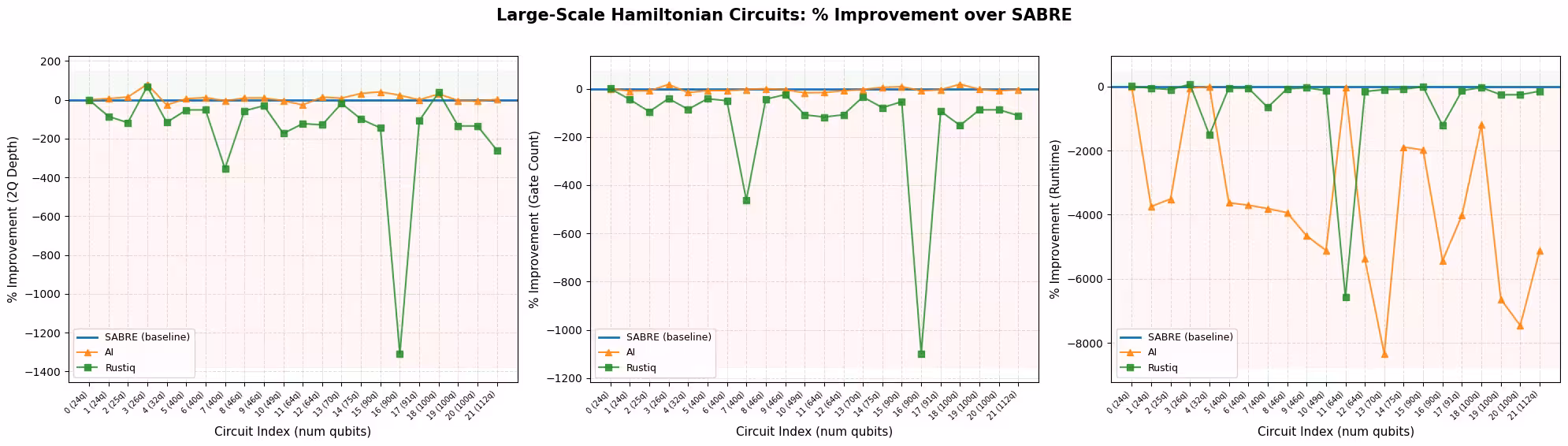
plot_pct_improvement_vs_sabre(
    results_large,
    "Large-Scale Hamiltonian Circuits",
)
plot_best_method_bars(results_large)

# Select circuit index 3 from the large-scale transpiled circuits
test_idx_large = 3
test_circuit_large = qc_large[test_idx_large]
print(
    f"Test circuit: {test_circuit_large.name}, {test_circuit_large.num_qubits} qubits"
)

tqc_methods_large = {
    "SABRE": tqc_sabre_large[test_idx_large],
    "AI": tqc_ai_large[test_idx_large],
    "Rustiq": tqc_rustiq_large[test_idx_large],
}

print(f"\nTranspilation metrics for circuit index {test_idx_large}:")
for method, tqc in tqc_methods_large.items():
    depth_2q = tqc.depth(lambda x: x.operation.num_qubits == 2)
    size = tqc.size()
    print(f"  {method:8s}  2Q depth={depth_2q:5d}  size={size:6d}")
Test circuit: tfim, 26 qubits

Transpilation metrics for circuit index 3:
  SABRE     2Q depth=  100  size=   489
  AI        2Q depth=   20  size=   402
  Rustiq    2Q depth=   31  size=   688
pm_mirror = generate_preset_pass_manager(
    optimization_level=0, backend=backend
)

for method, tqc in tqc_methods_large.items():
    # print the count ops for each circuit
    mirror = tqc.copy()
    mirror.compose(tqc.inverse(), inplace=True)
    mirror.measure_all()
    mirror = pm_mirror.run(mirror)
    print(f"\n{method} transpiled circuit:")
    print(tqc.count_ops())
    print(f"{method} mirror circuit count ops:")
    print(mirror.count_ops())
SABRE transpiled circuit:
OrderedDict({'sx': 211, 'rz': 163, 'cz': 104, 'x': 11})
SABRE mirror circuit count ops:
OrderedDict({'rz': 1170, 'sx': 422, 'cz': 208, 'measure': 156, 'x': 22, 'barrier': 1})

AI transpiled circuit:
OrderedDict({'sx': 165, 'rz': 162, 'cz': 68, 'x': 7})
AI mirror circuit count ops:
OrderedDict({'rz': 984, 'sx': 330, 'measure': 156, 'cz': 136, 'x': 14, 'barrier': 1})

Rustiq transpiled circuit:
OrderedDict({'sx': 316, 'rz': 225, 'cz': 140, 'x': 7})
Rustiq mirror circuit count ops:
OrderedDict({'rz': 1714, 'sx': 632, 'cz': 280, 'measure': 156, 'x': 14, 'barrier': 1})
# Build mirror circuits and submit to real hardware
# The inverse may introduce gates (e.g., sxdg) not in the backend's
# basis gate set, so we re-transpile the mirror circuit.
pm_mirror = generate_preset_pass_manager(
    optimization_level=0, backend=backend
)

shots_hw = 10000
hw_jobs = {}

for method, tqc in tqc_methods_large.items():
    mirror = tqc.copy()
    mirror.compose(tqc.inverse(), inplace=True)
    mirror.measure_all()

    # Re-transpile at opt level 0 to decompose into basis gates
    # without changing the layout or routing
    mirror = pm_mirror.run(mirror)

    sampler = SamplerV2(mode=backend)
    sampler.options.environment.job_tags = ["TUT_CMHSC"]
    job = sampler.run([mirror], shots=shots_hw)
    hw_jobs[method] = job
    print(f"{method}: submitted job {job.job_id()}")
SABRE: submitted job d8gvgq66983c73dqe5og
AI: submitted job d8gvgqe6983c73dqe5pg
Rustiq: submitted job d8gvgqm6983c73dqe5q0
# Retrieve results and compute fidelities
fidelities_large = {}

for method, job in hw_jobs.items():
    result = job.result()
    counts = result[0].data.meas.get_counts()

    n_qubits = backend.num_qubits
    all_zeros = "0" * n_qubits
    fidelity = counts.get(all_zeros, 0) / shots_hw
    fidelities_large[method] = fidelity
    print(
        f"{method:8s}  P(|00...0>) = {fidelity:.4f}  ({counts.get(all_zeros, 0)}/{shots_hw})"
    )
SABRE     P(|00...0>) = 0.0005  (5/10000)
AI        P(|00...0>) = 0.3267  (3267/10000)
Rustiq    P(|00...0>) = 0.1845  (1845/10000)
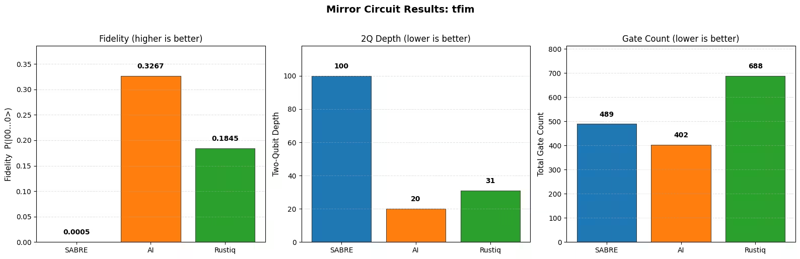
plot_mirror_results(
    tqc_methods_large, fidelities_large, test_circuit_large.name
)
コンパイル結果の分析
上記のベンチマークでは、Hamlibコレクションのハミルトニアンシミュレーション回路について、小規模と大規模の両方のスケールでSABRE、AI搭載トランスパイラ、Rustiqを比較しています。
2量子ビット深さとGate数
大規模においては、SABREとAI搭載トランスパイラが最も強力な2手法であり、それぞれ異なるメトリクスでリードしています。メトリクスごとの最良手法グラフが示すように、SABREは大部分の回路で最もGate数が少なく、ほぼすべての回路で最速の手法です。これは挿入されたSWAPゲートを最小化するように設計されたヒューリスティックと、最近のレイアウトおよびルーティングの最適化と一致しています。AI搭載トランスパイラは大部分の回路で最も低い2量子ビット深さを達成しており、これは回路深さをターゲットとする強化学習の目標関数の一部と一致しています。要約表も同じ分断を反映しています:SABREはより低い平均Gate数を、AIトランスパイラはより低い平均2量子ビット深さを持っています。両手法とも回路全体にわたって一貫性があり、信頼性があります。
PauliEvolutionGate合成のために特別に構築されたRustiqは、大規模回路の一部でのみ単独での最良結果を生成します。その平均メトリクスは、コンパイル比較プロットに大きなスパイクとして見える少数の重大な外れ値によって大きく歪められており、Rustiqが他の手法よりも大幅に高い深さとGate数を生成しています。これらの外れ値なしでは、平均性能はSABREおよびAI搭載トランスパイラにはるかに近くなるでしょう。
重要な観察点は、すべての回路で単一の手法が支配しているわけではないということです。各手法は特定のケースで他の手法を上回るため、利用可能なすべてのツールを試し、各回路に対して最良の結果を選択する価値があります。
実行時間
SABREは一貫して最速の手法です。Rustiqは一般的に同様の速度で動作しますが、コンパイルに著しく長い時間がかかる外れ値が発生することがあります。これは特に大規模な結果で顕著であり、いくつかの回路がRustiqの実行時間を急増させます。これらの外れ値は平均実行時間に大きな影響を与えるため、中央値がRustiqのより代表的なまとめになる可能性があります。AI搭載トランスパイラは3つの中で最も遅く、より大きく複雑な回路では実行時間が著しく増加します。
ミラー回路の結果
ミラー回路実験は期待されるトレンドを確認しています:ノイズ下では、2量子ビット深さが低くGate数が少ない手法が高い忠実度を達成します。これはノイズを含むシミュレータ(小規模)と実際のハードウェア(大規模)の両方で成立します。
各ミラー回路プロットは集計ではなく単一の回路を反映していることに留意してください。上記のハードウェア例では1つの26Qubittfim回路を使用しており、これはSABREがAI搭載トランスパイラとRustiqよりもはるかに高い2量子ビット深さを生成するケースであるため、その忠実度は相応に大幅に低くなっています。これは広範な結果を代表するものではありません:大規模回路の全セットにわたって、SABREの2量子ビット深さは通常AI搭載トランスパイラに近く、2つの手法はそれぞれ異なるメトリクスでリードしています(AI搭載トランスパイラは2量子ビット深さで、SABREはGate数と実行時間で)。単一のミラー結果は1つの回路の2倍バージョンをテストするものであり、全体的な手法の品質に対する評決として読むべきではありません。
推奨事項
すべての回路に対して単一の最良のトランスパイル戦略は存在しません。最良の選択は回路の構造、最適化の目標、および利用可能なコンパイル時間の予算に依存します:
- SABREは推奨されるデフォルトです。高速で信頼性が高く、幅広い回路で優れた結果を生成します。さらなるチューニングには、ユーザーがレイアウトとルーティングのトライアルを増やすことができます(SABREの最適化チュートリアルを参照)。
- AI搭載トランスパイラは、コンパイル時間が制約でない場合、特に2量子ビット深さの最小化が優先事項のときに試す価値があります:このベンチマークの大規模回路の大部分で最も低い2量子ビット深さを達成しました。
- Rustiqは
PauliEvolutionGate回路のために特別に構築されており、特に小規模回路で非常に低い深さと低いGate数の解を見つけることができます。大規模回路では時に大幅に大きな結果を生成することがあるため、デフォルトとして使用するのではなく、試すべき複数の手法の1つとして使用するのが最善です。
実際には、利用可能なすべての手法を実行し、各回路に対して最良の結果を選択することが最善のアプローチです。複数の手法を試すコンパイルオーバーヘッドは、実際のハードウェアでの実行品質の潜在的な改善と比べれば小さいものです。
次のステップ
このチュートリアルが役立った場合は、以下にも関心を持つかもしれません:
参考文献
[1] "LightSABRE: A Lightweight and Enhanced SABRE Algorithm". H. Zou, M. Treinish, K. Hartman, A. Ivrii, J. Lishman et al. https://arxiv.org/abs/2409.08368
[2] "Practical and efficient quantum circuit synthesis and transpiling with Reinforcement Learning". D. Kremer, V. Villar, H. Paik, I. Duran, I. Faro, J. Cruz-Benito et al. https://arxiv.org/abs/2405.13196
[3] "Pauli Network Circuit Synthesis with Reinforcement Learning". A. Dubal, D. Kremer, S. Martiel, V. Villar, D. Wang, J. Cruz-Benito et al. https://arxiv.org/abs/2503.14448
[4] "Faster and shorter synthesis of Hamiltonian simulation circuits". T. Goubault de Brugiere, S. Martiel et al. https://arxiv.org/abs/2404.03280