Qiskit AI搭載トランスパイラの紹介
推定使用時間:IBM Heron上で5分(注意:これはあくまで推定値です。実際の実行時間は異なる場合があります。)
学習の目標
このチュートリアルを通じて、ユーザーは以下について理解できます:
- 標準トランスパイラのドロップイン置き換えとして AI 搭載 Transpiler(
generate_ai_pass_manager)を使用する方法 - 2 Qubit 深度、Gate 数、トランスパイレーション時間の観点で AI 搭載 Transpiler がデフォルト Transpiler と比較してどうか
- ハードウェア実行によりトランスパイレーション品質を評価するためのミラー Circuit の使用方法
前提条件
このチュートリアルを進める前に、以下のトピックに精通していることを推奨します:
背景
Qiskit AI 搭載 Transpiler は、SABRE のような従来のヒューリスティック手法よりも短くハードウェア効率の高い Circuit を生成できる機械学習ベースのトランスパイレーション・パスを導入します。短い Circuit は累積ノイズが少なく、実際の量子ハードウェア上での結果品質を直接向上させます。
このチュートリアルでは、2 つのトランスパイレーション戦略を比較します:
| 戦略 | API |
|---|---|
| デフォルト | generate_preset_pass_manager(optimization_level=3, ...) |
| AI | generate_ai_pass_manager(optimization_level=1, ai_optimization_level=3, ...) |
各戦略について 2 Qubit Gate 深度、総 Gate 数、トランスパイレーション実行時間 の 3 つの指標を測定します。
AI 搭載 Transpiler のベンチマーク
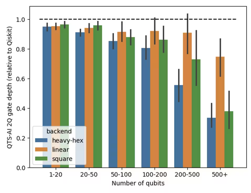
ベンチマーク・テストでは、AI 搭載 Transpiler は標準 Qiskit Transpiler と比較して、一貫してより浅く高品質な Circuit を生成しました。これらのテストでは、generate_preset_pass_manager で設定された Qiskit のデフォルト・パスマネージャー戦略を使用しました。このデフォルト戦略は多くの場合効果的ですが、大規模または複雑な Circuit では困難が生じることがあります。一方、AI 搭載パスは、IBM Quantum® ハードウェアの heavy-hex トポロジーにトランスパイルする場合、大規模回路(100 Qubit 以上)において 2 Qubit Gate 数の平均 24% 削減と Circuit 深度の平均 36% 削減を達成しました。これらのベンチマークの詳細については、こちらのブログを参照してください。
このチュートリアルでは、AI パスの主な利点と従来の手法との比較について解説します。
要件
このチュートリアルを始める前に、以下がインストールされていることを確認してください:
- Qiskit SDK v2.0 以降、visualization サポート付き
- Qiskit Runtime(
pip install qiskit-ibm-runtime)v0.22 以降 - AI ローカルモード付き Qiskit IBM Transpiler(
pip install 'qiskit-ibm-transpiler[ai-local-mode]') - Qiskit Aer(
pip install qiskit-aer)
セットアップ
# Added by doQumentation — required packages for this notebook
!pip install -q matplotlib qiskit qiskit-aer qiskit-ibm-runtime qiskit-ibm-transpiler
from qiskit import QuantumCircuit
from qiskit.circuit.random import random_circuit
from qiskit.transpiler import generate_preset_pass_manager
from qiskit_ibm_runtime import QiskitRuntimeService, SamplerV2
from qiskit_ibm_transpiler import generate_ai_pass_manager
from qiskit_aer import AerSimulator
from qiskit_aer.noise import NoiseModel, depolarizing_error
import matplotlib.pyplot as plt
from statistics import mean, stdev
import time
import logging

seed = 42

def transpile_with_metrics(pass_manager, circuit):
    """Transpile a circuit and return the result along with key metrics."""
    start = time.time()
    qc_out = pass_manager.run(circuit)
    elapsed = time.time() - start

    depth_2q = qc_out.depth(lambda x: x.operation.num_qubits == 2)
    gate_count = qc_out.size()

    return qc_out, {
        "depth_2q": depth_2q,
        "gate_count": gate_count,
        "time_s": round(elapsed, 3),
    }

def remap_to_contiguous(tqc):
    """Remap a transpiled circuit to use contiguous qubit indices.

    Transpiled circuits target specific physical qubits (e.g., qubit 45, 67)
    on a large backend. This remaps them to 0, 1, 2, ... so Aer only
    simulates the active qubits."""
    active = sorted(
        {tqc.find_bit(q).index for inst in tqc.data for q in inst.qubits}
    )
    qubit_map = {old: new for new, old in enumerate(active)}
    new_qc = QuantumCircuit(len(active))
    for inst in tqc.data:
        old_indices = [tqc.find_bit(q).index for q in inst.qubits]
        new_qc.append(inst.operation, [qubit_map[i] for i in old_indices])
    return new_qc

def build_mirror_circuit(tqc, simulate=True):
    """Build a mirror circuit: U followed by U-dagger, with measurements.

    The expected output is always |0...0>, so measuring the survival
    probability reveals how much noise each transpilation strategy adds.

    Args:
        tqc: A transpiled circuit.
        simulate: If True (default), remap to contiguous qubits so Aer
            only simulates the active qubits. If False, keep the full
            physical layout for hardware execution."""
    if simulate:
        tqc = remap_to_contiguous(tqc)
    mirror = tqc.compose(tqc.inverse())
    mirror.measure_all()
    return mirror

def print_summary(results):
    """Print a summary of each metric as mean +/- stdev across all circuits,
    along with the mean percentage improvement of AI over Default."""
    metrics = [
        ("Depth 2Q", "Depth 2Q (Default)", "Depth 2Q (AI)"),
        ("Gate Count", "Gate Count (Default)", "Gate Count (AI)"),
        ("Time (s)", "Time (Default)", "Time (AI)"),
    ]
    header = (
        f"{'Metric':<12}{'Default (mean +/- std)':>24}"
        f"{'AI (mean +/- std)':>22}{'AI % improvement':>22}"
    )
    print(header)
    print("-" * len(header))
    for label, col_def, col_ai in metrics:
        defaults = [r[col_def] for r in results]
        ais = [r[col_ai] for r in results]
        pct = [(d - a) / d * 100 for d, a in zip(defaults, ais)]
        default_str = f"{mean(defaults):.1f} +/- {stdev(defaults):.1f}"
        ai_str = f"{mean(ais):.1f} +/- {stdev(ais):.1f}"
        pct_str = f"{mean(pct):+.1f}% +/- {stdev(pct):.1f}%"
        print(f"{label:<12}{default_str:>24}{ai_str:>22}{pct_str:>22}")

def plot_metrics_and_pct(results, title_prefix):
    """Plot metric comparisons and percentage improvement of AI over Default."""
    qubits = [r["Qubits"] for r in results]
    metrics = [
        ("Depth 2Q (Default)", "Depth 2Q (AI)", "Two-Qubit Depth"),
        ("Gate Count (Default)", "Gate Count (AI)", "Gate Count"),
        ("Time (Default)", "Time (AI)", "Transpilation Time"),
    ]

    # Row 1: raw metric comparison
    fig, axs = plt.subplots(1, 3, figsize=(21, 5))
    fig.suptitle(
        f"{title_prefix}: Metric Comparison",
        fontsize=15,
        fontweight="bold",
        y=1.02,
    )
    for ax, (col_def, col_ai, label) in zip(axs, metrics):
        ax.plot(qubits, [r[col_def] for r in results], "o-", label="Default")
        ax.plot(qubits, [r[col_ai] for r in results], "s-", label="AI")
        ax.set_title(label)
        ax.set_xlabel("Number of Qubits")
        ax.set_ylabel(label)
        ax.legend()
    plt.tight_layout()
    plt.show()

    # Row 2: percentage improvement
    fig, axs = plt.subplots(1, 3, figsize=(21, 5))
    fig.suptitle(
        f"{title_prefix}: % Improvement of AI over Default",
        fontsize=15,
        fontweight="bold",
        y=1.02,
    )
    for ax, (col_def, col_ai, label) in zip(axs, metrics):
        pct = [(r[col_def] - r[col_ai]) / r[col_def] * 100 for r in results]
        ax.axhline(
            0, color="#1f77b4", linewidth=2, label="Default (baseline)"
        )
        ax.plot(qubits, pct, "s-", color="#ff7f0e", label="AI")
        ax.fill_between(qubits, 0, pct, alpha=0.15, color="#ff7f0e")
        ax.set_title(label)
        ax.set_xlabel("Number of Qubits")
        ax.set_ylabel("% Improvement")
        ax.legend()
    plt.tight_layout()
    plt.show()

# Suppress verbose AI-powered transpiler logs
logging.getLogger(
    "qiskit_ibm_transpiler.wrappers.ai_local_synthesis"
).setLevel(logging.WARNING)
小規模シミュレーターの例
ステップ 1: 古典的な入力を量子問題にマッピングする
深度 4 のランダムな Circuit を 20 個生成します。Qubit 数は 6 から 25 の範囲です。これらの Circuit が、トランスパイレーション戦略を比較するためのテストケースとなります。
num_circuits_sim = 20
depth_sim = 4
qubit_range_sim = list(range(6, 26))

circuits_sim = [
    # We have only two qubit gates, as those test how well the transpiler can optimize the circuit.
    random_circuit(
        num_qubits=n,
        depth=depth_sim,
        max_operands=2,
        num_operand_distribution={2: 1},
        seed=seed + i,
    )
    for i, n in enumerate(qubit_range_sim)
]

print(
    f"Created {len(circuits_sim)} circuits with qubit counts: {qubit_range_sim}"
)
circuits_sim[0].draw(output="mpl", fold=-1)
Created 20 circuits with qubit counts: [6, 7, 8, 9, 10, 11, 12, 13, 14, 15, 16, 17, 18, 19, 20, 21, 22, 23, 24, 25]

ステップ 2: 量子ハードウェア実行のための問題の最適化
選択した Backend のデフォルト(SABRE)パスマネージャーを構築します。両方のトランスパイレーション戦略は、Backend の完全なカップリング・マップをターゲットとします。シミュレーション・ステップでは remap_to_contiguous を使用して、トランスパイルされた各 Circuit をアクティブな Qubit のみにリマップするため、Aer はデバイス全体ではなくその Qubit のみをシミュレートします。
service = QiskitRuntimeService()
backend = service.least_busy(
    min_num_qubits=100, operational=True, simulator=False
)

pm_default_sim = generate_preset_pass_manager(
    optimization_level=3,
    backend=backend,
    seed_transpiler=seed,
)
results_sim = []

for i, qc in enumerate(circuits_sim):
    n = qubit_range_sim[i]

    qc_default, m_default = transpile_with_metrics(pm_default_sim, qc)

    # Create a fresh AI pass manager each iteration to avoid stale layout state
    pm_ai = generate_ai_pass_manager(
        optimization_level=1,
        ai_optimization_level=3,
        backend=backend,
    )
    qc_ai, m_ai = transpile_with_metrics(pm_ai, qc)

    results_sim.append(
        {
            "Qubits": n,
            "Depth 2Q (Default)": m_default["depth_2q"],
            "Depth 2Q (AI)": m_ai["depth_2q"],
            "Gate Count (Default)": m_default["gate_count"],
            "Gate Count (AI)": m_ai["gate_count"],
            "Time (Default)": m_default["time_s"],
            "Time (AI)": m_ai["time_s"],
        }
    )

print_summary(results_sim)
Fetching 4 files: 0%| | 0/4 [00:00<?, ?it/s]
Metric        Default (mean +/- std)     AI (mean +/- std)      AI % improvement
--------------------------------------------------------------------------------
Depth 2Q               33.0 +/- 12.9          26.4 +/- 8.0      +15.8% +/- 17.6%
Gate Count           522.0 +/- 266.0       560.5 +/- 279.1        -9.0% +/- 9.0%
Time (s)                 0.0 +/- 0.0           0.2 +/- 0.1    -893.6% +/- 362.9%
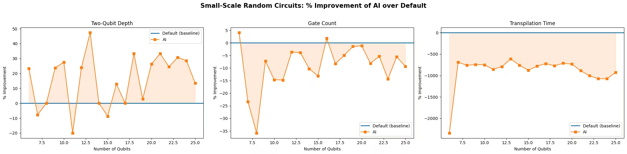
サマリーテーブルは、20 個の Circuit 全体における各指標の平均と標準偏差、および AI 搭載 Transpiler のデフォルトに対する平均改善率を示しています。正の値は AI 搭載 Transpiler の方が良い結果を出したことを、負の値はデフォルトの方が優れていたことを示します。
この小規模な例では、AI 搭載 Transpiler は平均して約 16% 低い 2 Qubit 深度を達成していますが、その代わりに約 9% 高い Gate 数というコストが生じています。これは、2 つの戦略を選択する際の重要なトレードオフを浮き彫りにしています。AI 搭載 Transpiler は深度削減(2 Qubit Gate の連続レイヤーの削減)を優先するのに対し、デフォルト Transpiler(SABRE)は総 Gate 数の最小化(SWAP 挿入の削減)を優先します。アプリケーションによって、どちらの指標がより重要かが異なります。
plot_metrics_and_pct(results_sim, "Small-Scale Random Circuits")
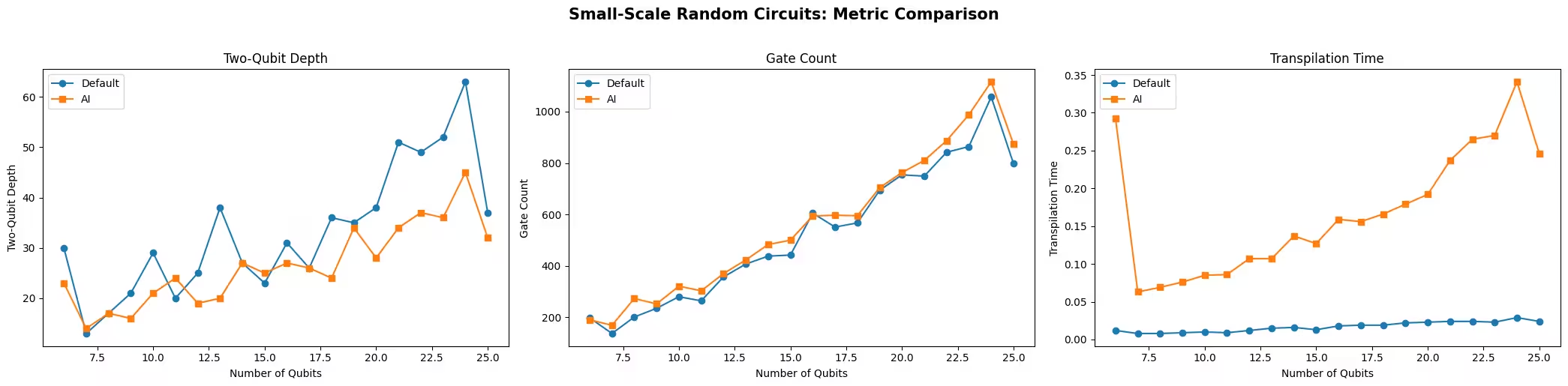
2 Qubit 深度: AI 搭載 Transpiler は一般的により低い 2 Qubit 深度の Circuit を生成します。深度は AI ルーティング・モデルが最適化するよう訓練されている主要な指標の一つであり、ほとんどの Circuit サイズで改善が見られますが、SABRE が個々の Circuit で同等か上回ることもあります。
Gate 数: このスケールでは結果がほぼ拮抗しており、SABRE が全体的にわずかに優位です。SABRE のルーティング・ヒューリスティックは挿入される SWAP Gate の数を最小化するよう設計されており、これが Gate 数を直接削減します。小規模の Circuit サイズでは差は小さいです。
トランスパイレーション時間: SABRE の実行時間は Qubit 数に関わらずほぼ一定なため、このスケールでは Circuit サイズがトランスパイレーション時間にほとんど影響しません。SABRE のコア・ルーティング・ロジックは高度に最適化されています(主に Rust で実装)。AI 搭載 Transpiler はかなり時間がかかり、Circuit サイズとともにスケールしますが、インタラクティブな使用において絶対的な時間は合理的な範囲に収まっています。
ステップ 3: Qiskit プリミティブを使用して実行する
トランスパイレーションが Circuit の忠実度に与える影響を評価するために、10 Qubit のケースからミラー Circuit を構築し、単純なノイズ・モデルを使って Aer シミュレーターで実行します。ミラー Circuit の期待される出力は常に全ゼロのビット列であるため、 を測定する確率は各トランスパイレーション戦略がどれだけ忠実度を保持するかを示します。
# Use the 10-qubit circuit (index where qubits == 10)
idx_10q = qubit_range_sim.index(10)

qc_10q = circuits_sim[idx_10q]
qc_default_10q, _ = transpile_with_metrics(pm_default_sim, qc_10q)

pm_ai = generate_ai_pass_manager(
    optimization_level=1,
    ai_optimization_level=3,
    backend=backend,
)
qc_ai_10q, _ = transpile_with_metrics(pm_ai, qc_10q)

tqc_methods = {
    "Default": qc_default_10q,
    "AI": qc_ai_10q,
}

print(
    f"Default: depth {qc_default_10q.depth()}, gates {qc_default_10q.size()}"
)
print(f"AI:      depth {qc_ai_10q.depth()}, gates {qc_ai_10q.size()}")
Default: depth 84, gates 280
AI:      depth 91, gates 343
# Build a simple depolarizing noise model
noise_model = NoiseModel()
noise_model.add_all_qubit_quantum_error(
    depolarizing_error(0.001, 1),
    ["sx", "x", "rz"],  # ~0.1% per 1Q gate
)
noise_model.add_all_qubit_quantum_error(
    depolarizing_error(0.01, 2),
    ["cx", "ecr"],  # ~1% per 2Q gate
)

aer_sim = AerSimulator(noise_model=noise_model)

shots = 10000
survival_probs = {}

for method, tqc in tqc_methods.items():
    mirror = build_mirror_circuit(tqc, simulate=True)

    sampler = SamplerV2(mode=aer_sim)
    job = sampler.run([mirror], shots=shots)
    counts = job.result()[0].data.meas.get_counts()

    all_zeros = "0" * mirror.num_qubits
    survival = counts.get(all_zeros, 0) / shots
    survival_probs[method] = survival
    print(
        f"{method:8s}  P(|00...0>) = {survival:.4f}  ({counts.get(all_zeros, 0)}/{shots})"
    )
Default   P(|00...0>) = 0.8460  (8460/10000)
AI        P(|00...0>) = 0.8121  (8121/10000)
単純な脱分極ノイズ・モデルを使って Aer シミュレーターで両方のミラー Circuit を実行しました。生存確率(全ゼロのビット列を返すショットの割合)は、各トランスパイレーション戦略がどれだけのノイズを導入するかを定量化します。
ステップ 4: 後処理と希望する古典的な形式での結果の返却
両方の実行から全ゼロのビット列を測定する確率を抽出します。生存確率が高いほど忠実度が高く、トランスパイレーションが導入するノイズが少ないことを意味します。以下のプロットは補数である 1 - P(|0...0>) を示しているため、低いバーほど忠実度が高く、誤差の小さな差が見やすくなっています。
# Plot 1 - P(|0...0>), the probability of an erroneous (non-zero) outcome.
# A lower bar means the transpilation introduced less noise.
error_probs = {method: 1 - p for method, p in survival_probs.items()}

fig, ax = plt.subplots(figsize=(6, 4))
ax.bar(
    error_probs.keys(),
    error_probs.values(),
    color=["steelblue", "coral"],
)
ax.set_ylabel("1 - P(|0...0>)")
ax.set_title("Mirror Circuit Error (10-qubit, Aer Simulator)")
ax.set_ylim(0, 1)
plt.tight_layout()
plt.show()

この場合、デフォルト Transpiler はこの特定の 10 Qubit のインスタンスに対してより浅く小さな Circuit を生成したため、より高い忠実度は予想通りです。回路ごとの結果は異なります。上のサマリーテーブルが示すように、AI 搭載 Transpiler の優位性は個々の Circuit ごとではなく平均的に低い 2 Qubit 深度にあります。どちらの戦略がより高い忠実度をもたらすかは、各指標の差の大きさ、ハードウェアのノイズ特性、Circuit の構造によって異なります。均一な脱分極ノイズ・モデルでは、総 Gate 数は深度単独よりも累積誤差に直接的な影響を与えることが多いです。
大規模ハードウェアの例
ステップ 1〜4
ここでは、これらの詳細すべてをより大きなスケールで明確なワークフローにまとめ、実際の量子ハードウェア上で実行します。
以下のコードは、深度 8 のランダムな Circuit を 25 個生成します。Qubit 数は 26 から 50 の範囲です。これらの Circuit は両方の戦略でトランスパイルされ、同じ指標が収集されます。次に 26 Qubit のケースからミラー Circuit を構築し、実際の Backend に送信します。
# -------------------------Step 1-------------------------
num_circuits_hw = 25
depth_hw = 8
qubit_range_hw = list(range(26, 51))

circuits_hw = [
    # We have only two qubit gates, as those test how well the transpiler can optimize the circuit.
    random_circuit(
        num_qubits=n,
        depth=depth_hw,
        max_operands=2,
        num_operand_distribution={2: 1},
        seed=seed + i,
    )
    for i, n in enumerate(qubit_range_hw)
]

print(
    f"Created {len(circuits_hw)} circuits with qubit counts: {qubit_range_hw}"
)
Created 25 circuits with qubit counts: [26, 27, 28, 29, 30, 31, 32, 33, 34, 35, 36, 37, 38, 39, 40, 41, 42, 43, 44, 45, 46, 47, 48, 49, 50]
# -------------------------Step 2-------------------------
pm_default = generate_preset_pass_manager(
    optimization_level=3,
    backend=backend,
    seed_transpiler=seed,
)

results_hw = []

for i, qc in enumerate(circuits_hw):
    n = qubit_range_hw[i]

    qc_default, m_default = transpile_with_metrics(pm_default, qc)

    # Create a fresh AI pass manager each iteration to avoid stale layout state
    pm_ai = generate_ai_pass_manager(
        optimization_level=1,
        ai_optimization_level=3,
        backend=backend,
    )
    qc_ai, m_ai = transpile_with_metrics(pm_ai, qc)

    results_hw.append(
        {
            "Qubits": n,
            "Depth 2Q (Default)": m_default["depth_2q"],
            "Depth 2Q (AI)": m_ai["depth_2q"],
            "Gate Count (Default)": m_default["gate_count"],
            "Gate Count (AI)": m_ai["gate_count"],
            "Time (Default)": m_default["time_s"],
            "Time (AI)": m_ai["time_s"],
        }
    )

print_summary(results_hw)
Metric        Default (mean +/- std)     AI (mean +/- std)      AI % improvement
--------------------------------------------------------------------------------
Depth 2Q              217.4 +/- 50.4        191.0 +/- 35.6      +10.9% +/- 10.7%
Gate Count         4513.3 +/- 1394.3     5227.1 +/- 1536.4       -16.4% +/- 5.8%
Time (s)                 0.1 +/- 0.0           3.5 +/- 1.5   -3588.2% +/- 643.6%
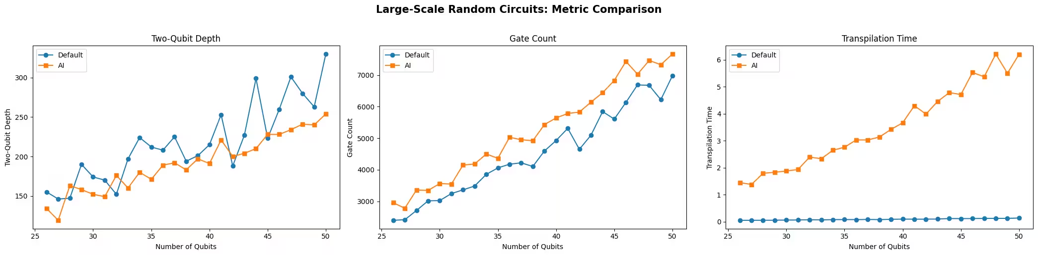
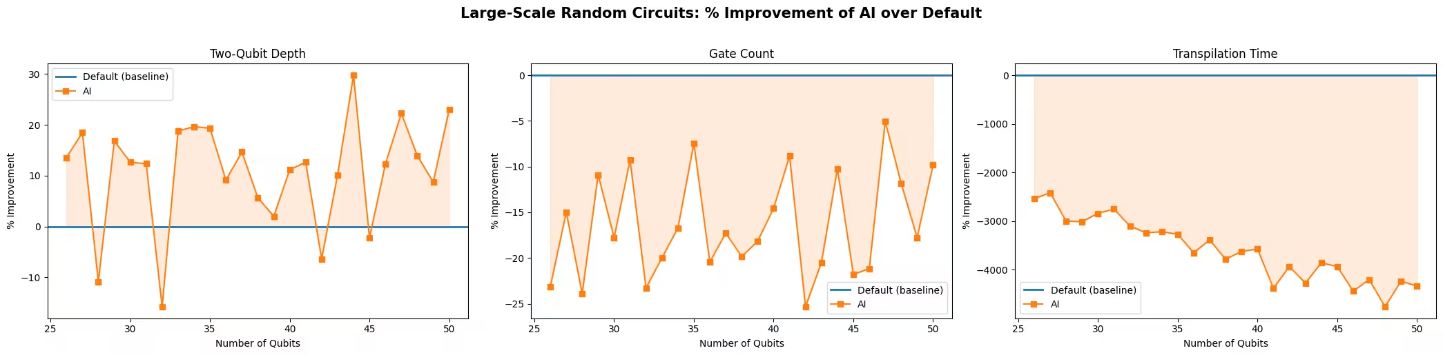
plot_metrics_and_pct(results_hw, "Large-Scale Random Circuits")
# -------------------------Step 3-------------------------
# Build mirror circuits from the 26-qubit case
idx_26q = qubit_range_hw.index(26)

qc_26q = circuits_hw[idx_26q]
qc_default_26q, _ = transpile_with_metrics(pm_default, qc_26q)

pm_ai = generate_ai_pass_manager(
    optimization_level=1,
    ai_optimization_level=3,
    backend=backend,
)
qc_ai_26q, _ = transpile_with_metrics(pm_ai, qc_26q)

mirror_default_hw = build_mirror_circuit(qc_default_26q, simulate=False)
mirror_ai_hw = build_mirror_circuit(qc_ai_26q, simulate=False)

# Re-transpile to basis gates (the inverse can introduce gates like sxdg)
pm_basis = generate_preset_pass_manager(
    optimization_level=0,
    backend=backend,
)
mirror_default_hw = pm_basis.run(mirror_default_hw)
mirror_ai_hw = pm_basis.run(mirror_ai_hw)

print(
    f"Mirror circuit (Default): depth {mirror_default_hw.depth()}, gates {mirror_default_hw.size()}"
)
print(
    f"Mirror circuit (AI):      depth {mirror_ai_hw.depth()}, gates {mirror_ai_hw.size()}"
)

# Submit to real hardware
sampler_hw = SamplerV2(mode=backend)
sampler_hw.options.environment.job_tags = ["TUT_AITI"]

shots_hw = 500000
job_hw = sampler_hw.run([mirror_default_hw, mirror_ai_hw], shots=shots_hw)
print(f"Job submitted: {job_hw.job_id()}")
Mirror circuit (Default): depth 1577, gates 9672
Mirror circuit (AI):      depth 1235, gates 11092
Job submitted: d8gt7vm6983c73dqbg0g
# -------------------------Step 4-------------------------
result_hw = job_hw.result()

survival_probs_hw = {}
for i, method in enumerate(["Default", "AI"]):
    counts = result_hw[i].data.meas.get_counts()
    mirror = [mirror_default_hw, mirror_ai_hw][i]
    all_zeros = "0" * mirror.num_qubits
    survival = counts.get(all_zeros, 0) / shots_hw
    survival_probs_hw[method] = survival
    print(
        f"{method:8s}  P(|00...0>) = {survival:.4f}  ({counts.get(all_zeros, 0)}/{shots_hw})"
    )

# Plot 1 - P(|0...0>), the probability of an erroneous (non-zero) outcome.
# A lower bar means the transpilation introduced less noise.
error_probs_hw = {method: 1 - p for method, p in survival_probs_hw.items()}

fig, ax = plt.subplots(figsize=(6, 4))
ax.bar(
    error_probs_hw.keys(),
    error_probs_hw.values(),
    color=["steelblue", "coral"],
)
ax.set_ylabel("1 - P(|0...0>)")
ax.set_title(f"Mirror Circuit Error (26-qubit, {backend.name})")
ax.set_ylim(0, 1)
plt.tight_layout()
plt.show()
Default   P(|00...0>) = 0.0005  (239/500000)
AI        P(|00...0>) = 0.0050  (2516/500000)

結果の分析
大規模な結果は、より要求の高いスケールで小規模の例で観察されたトレンドを強化しています。
2 Qubit 深度: AI 搭載 Transpiler は引き続き Circuit サイズの全範囲にわたって著しく低い 2 Qubit 深度を達成しています。深度最適化は AI ルーティング・モデルが訓練されている主要な目標の一つであり、ルーティング問題がヒューリスティック手法にとって困難になる大きな Qubit 数においてその優位性がより顕著になります。
Gate 数: デフォルト Transpiler(SABRE)はこの範囲のすべての Circuit サイズで一貫してより少ない Gate 数の Circuit を生成します。SABRE のヒューリスティックは Gate 数を最小化するよう特に設計されており、このスケールではその優位性が明確かつ均一です。
トランスパイレーション時間: トランスパイレーション時間の差は大きなスケールで広がります。SABRE はほぼ一定のままですが、AI 搭載 Transpiler の実行時間はより急激に増加します。それでも、AI 搭載 Transpiler の実行時間はほとんどのワークフローで実用的な範囲に収まっています。
ミラー Circuit の忠実度: 両方の手法はこのスケールでは生存確率が 1% をはるかに下回り、使用可能なシグナルがほとんど残りません。総 Gate 数が約 10,000、2 Qubit 深度が 1,000 を超えると、ミラー Circuit 全体に蓄積された脱分極ノイズがシグナルの大部分を圧倒します。これはミラー Circuit アプローチの重要な限界を浮き彫りにしています:シンプルで古典シミュレーションを必要としない一方で、両方の手法がノイズ・フロアに近づき、残った小さなシグナルが蓄積誤差に支配される大規模または深い Circuit にはうまくスケールしません。
これらの結果は AI 搭載 Transpiler の有効性を強調していますが、その制限事項にも注意することが重要です。AI 合成手法は現在、特定のカップリング・マップに対してのみ利用可能であり、より広範な適用性が制限される可能性があります。この制約は、異なるシナリオでの使用を評価する際に考慮する必要があります。
次のステップ
この研究が興味深いと思われた方は、以下の資料をご覧ください: