Kipu QuantumのRimay Quantum Feature Extractionによる信用リスクの分類
Qiskit Functionsは、IBM Quantum® Premium Plan、Flex Plan、On-Prem(IBM Quantum Platform API経由)Planのユーザーのみが利用できる実験的な機能です。プレビューリリースの状態であり、変更される可能性があります。
使用量の目安: Nighthawk r2プロセッサーで2分。(注: これはあくまで目安です。実際の実行時間は異なる場合があります。)
学習目標
-
カテゴリー列と数値列を含む表形式データを、Rimay Qiskit Functionのために準備する。
-
訓練データで量子特徴マッピングをフィットし、同じ実行でテストデータをマッピングする。
-
量子変換された特徴量だけの場合と、元の特徴量と組み合わせた場合とで、古典モデルを訓練する。
-
結果を純粋に古典的なベースラインと比較する。
前提条件
このチュートリアルを始める前に、以下のトピックに慣れておく必要があります。
-
scikit-learnによる教師あり分類
背景
産業界の多くの機械学習の問題は、小規模から中規模の表形式データセットを扱い、データを追加することができず、モデルの精度が頭打ちになります。信用リスクのスコアリングはその典型例です。貸し手は数十の属性を使って、申込者が与信を返済しそうかどうかを判断します。
Kipu QuantumのQiskit FunctionであるRimayは、このようなパイプラインに量子前処理のステップを追加します。これは、デジタル化された反断熱量子特徴抽出アルゴリズム [1] を実装しています。各入力特徴量は1つの量子ビットにマッピングされます。特徴量の値と特徴量間の相互情報量が、スピングラス・ハミルトニアンの局所場とカップリングを決めます。続いて反断熱ダイナミクスが量子系を低エネルギー状態へと発展させ、最後に測定される1体および2体の期待値が、新しい量子変換された特徴量になります。これらの特徴量は入力間の非線形な相関を捉えており、任意の古典モデルに入力できます。
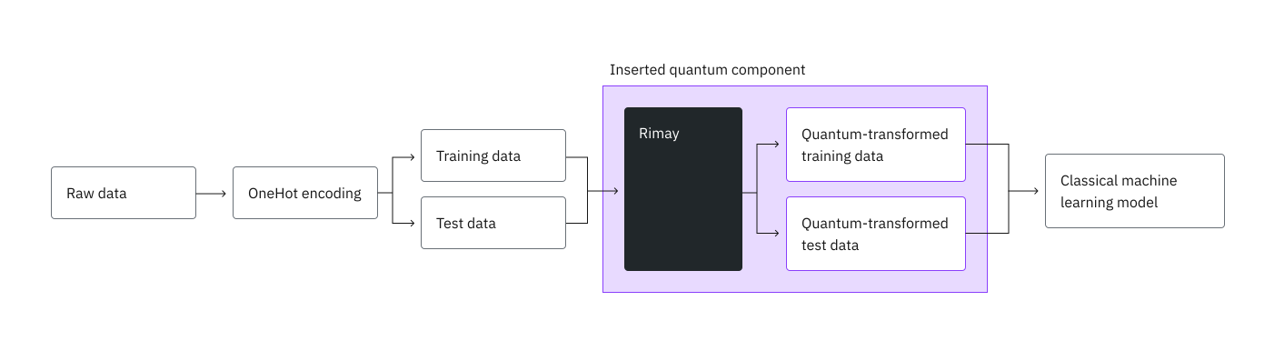
このチュートリアルでは、OpenMLのドイツ信用データセット [2](申込者1000人、属性20個)を使って、ランダムフォレスト分類器を訓練します。まず古典的なベースラインを確立し、次にデータをRimayに送り、最後に量子変換された特徴量だけの場合と、元の特徴量と組み合わせた場合とで、同じ種類のモデルを訓練します。
要件
このチュートリアルを始める前に、以下のパッケージがインストールされていることを確認してください。
-
IBM Quantum Computeクライアント(
pip install qiskit-ibm-runtime) -
Qiskit Functions(
pip install qiskit-ibm-catalog) -
scikit-learn(
pip install scikit-learn) -
pandas (
pip install pandas) -
Matplotlib (
pip install matplotlib)
Qiskit Functions CatalogのRimay関数へのアクセスも必要です。
セットアップ
パッケージをインポートし、2つのヘルパー関数を定義します。1つはランダムフォレストを学習する関数、もう1つはチュートリアル全体で使用する指標を計算する関数です。
# Added by doQumentation — installs the packages this notebook needs if they are missing
import importlib.util

_needed = {"matplotlib": "matplotlib", "numpy": "numpy", "pandas": "pandas", "qiskit_ibm_catalog": "qiskit-ibm-catalog", "sklearn": "scikit-learn"}
_missing = [pip for module, pip in _needed.items()
            if importlib.util.find_spec(module) is None]
# One at a time, so a package that fails to install does not block the others
for _pip in _missing:
    %pip install -q {_pip}
if not _missing:
    print("\u2713 All required packages are installed")
import matplotlib.pyplot as plt
import numpy as np
import pandas as pd
from qiskit_ibm_catalog import QiskitFunctionsCatalog
from sklearn.datasets import fetch_openml
from sklearn.ensemble import RandomForestClassifier
from sklearn.metrics import (
    accuracy_score,
    f1_score,
    precision_score,
    recall_score,
    roc_auc_score,
)
from sklearn.model_selection import train_test_split
from sklearn.preprocessing import OneHotEncoder

def train_random_forest(x, y, n_estimators, max_depth):
    """Train a random forest classifier with fixed hyperparameters."""
    model = RandomForestClassifier(
        n_estimators=n_estimators,
        max_depth=max_depth,
        min_samples_split=5,
        min_samples_leaf=1,
        max_features="sqrt",
        random_state=42,
        n_jobs=-1,
    )
    return model.fit(x, y)

def evaluate(model, x, y):
    """Return the classification metrics of a trained model on a test set."""
    y_pred = model.predict(x)
    y_proba = model.predict_proba(x)[:, 1]
    return {
        "Accuracy": accuracy_score(y, y_pred),
        "AUC": roc_auc_score(y, y_proba),
        "F1 score": f1_score(y, y_pred),
        "Precision": precision_score(y, y_pred),
        "Recall": recall_score(y, y_pred),
    }
IBM Quantum の認証情報を設定する
IBM Quantum Platform API キーで認証し、Rimay 関数を読み込んで、お使いのインスタンスで利用可能な最も空いている量子プロセッサーを選択します。
catalog = QiskitFunctionsCatalog(channel="ibm_quantum_platform")
rimay = catalog.load("kipu-quantum/rimay")

backend = catalog.least_busy(operational=True, simulator=False)
print(backend.name, backend.num_qubits)
ibm_fez 156
ステップ 1: 古典的な入力を量子問題にマッピングする
Rimay は数値の入力特徴量をそれぞれ1つの量子ビットにマッピングするため、最初のステップは生のテーブルを数値特徴量に変換することです。
データセットを読み込む
German credit データセットを OpenML から直接読み込みます。class 列にはラベルが入っており、good はクレジットを返済した申込者、bad は返済しなかった申込者を表します。
df = fetch_openml(data_id=31, as_frame=True).frame
print(df.shape)
df.head()
(1000, 21)
checking_status  duration                  credit_history  \
0              <0         6  critical/other existing credit
1        0<=X<200        48                   existing paid
2     no checking        12  critical/other existing credit
3              <0        42                   existing paid
4              <0        24              delayed previously

               purpose  credit_amount    savings_status employment  \
0             radio/tv           1169  no known savings        >=7
1             radio/tv           5951              <100     1<=X<4
2            education           2096              <100     4<=X<7
3  furniture/equipment           7882              <100     4<=X<7
4              new car           4870              <100     1<=X<4

   installment_commitment     personal_status other_parties  ...  \
0                       4         male single          none  ...
1                       2  female div/dep/mar          none  ...
2                       2         male single          none  ...
3                       2         male single     guarantor  ...
4                       3         male single          none  ...

   property_magnitude age  other_payment_plans   housing existing_credits  \
0         real estate  67                 none       own                2
1         real estate  22                 none       own                1
2         real estate  49                 none       own                1
3      life insurance  45                 none  for free                1
4   no known property  53                 none  for free                2

                  job num_dependents  own_telephone foreign_worker class
0             skilled              1            yes            yes  good
1             skilled              1           none            yes   bad
2  unskilled resident              2           none            yes  good
3             skilled              2           none            yes  good
4             skilled              2           none            yes   bad

[5 rows x 21 columns]
特徴量をエンコードする
ラベルを二値に変換し、13個のカテゴリ列をワンホットエンコードします。このコードは冗長な特徴量を避けるために各列の最初のカテゴリを削除し、結果として48個の数値特徴量が得られます。
y = (df["class"] == "good").astype(int)

features = df.drop(columns="class")
categorical_cols = [
    col for col in features.columns if features[col].dtype.name == "category"
]
encoder = OneHotEncoder(
    sparse_output=False, handle_unknown="ignore", drop="first"
)
encoded = pd.DataFrame(
    encoder.fit_transform(features[categorical_cols]),
    columns=encoder.get_feature_names_out(categorical_cols),
    index=features.index,
)
x = pd.concat([features.drop(columns=categorical_cols), encoded], axis=1)
print(f"{x.shape[1]} features")
48 features
学習セットとテストセットに分割する
申込者の20%をテストセットとして取り分けます。層化分割により、良好なクレジットと不良なクレジットの割合が両方のセットで等しく保たれます。
x_train, x_test, y_train, y_test = train_test_split(
    x, y, test_size=0.2, random_state=42, stratify=y
)
print(f"Training set: {x_train.shape}, test set: {x_test.shape}")
Training set: (800, 48), test set: (200, 48)
古典的なベースラインを確立する
古典的な特徴量でランダムフォレストを学習します。ステップ 4 では、量子変換された特徴量をこの指標と比較します。
baseline = train_random_forest(
    x_train, y_train, n_estimators=500, max_depth=12
)
results = {"Classical": evaluate(baseline, x_test, y_test)}
pd.DataFrame(results).T
Accuracy       AUC  F1 score  Precision    Recall
Classical     0.765  0.781071  0.845902   0.781818  0.921429
データを Rimay にアップロードする
Rimay は、関数にアップロードした CSV ファイルから入力を読み取ります。特徴量とラベルは別々のファイルに入れます。テストセットもアップロードすることで、Rimay は学習セットで適合させたものと同じマッピングでテストセットをマッピングします。
x_train.to_csv("x_train.csv", index=False)
y_train.to_csv("y_train.csv", index=False)
x_test.to_csv("x_test.csv", index=False)

for file_name in ("x_train.csv", "y_train.csv", "x_test.csv"):
    catalog.file_upload(file_name, rimay)
ステップ 2: 量子ハードウェアでの実行に向けて問題を最適化する
Rimay は選択したプロセッサー向けに回路を構築してトランスパイルするため、手動で最適化する回路はありません。次の制約の範囲内で、回路ごとのショット数を指定します。
-
各特徴量に量子ビットが1つ必要なので、プロセッサーにはデータセットの特徴量数以上の量子ビット数が必要です。
-
Rimay は、学習行とテスト行を合わせて、行ごとに1つの回路を実行します。1つのジョブで要求できる実行回数は最大1,000万回なので、行数に
shotsを掛けた値がこの上限内に収まる必要があります。
ジョブを送信する前に、両方の制限を確認してください。
ジョブは、回路がキューで待機する時間も含めて24時間以内に完了する必要があります。そうでない場合、結果が得られないまま停止されます。
shots = 5000

n_rows = len(x_train) + len(x_test)
n_features = x_train.shape[1]
print(f"Qubits needed: {n_features} of {backend.num_qubits} available")
print(f"Executions: {n_rows * shots:,} of 10,000,000 allowed")
Qubits needed: 48 of 156 available
Executions: 5,000,000 of 10,000,000 allowed
関数サイズを計算する
すべてのジョブは、S、M、L のいずれかの関数サイズで実行され、実行に使用される計算リソースが決まります。Rimay の場合、サイズはジョブがマッピングする行数(学習行とテスト行の合計)によって決まります。小さすぎるサイズを要求すると、ジョブはエラー 4600 で失敗します。サイズとその制限については、Rimay ガイドの関数サイズを参照してください。
次のセルでは、サイズ計算ツールを定義します。これはお使いのマシン上で実行され、渡したデータのみを読み取り、何も送信しません。
from os import PathLike
from typing import Any, Literal, Sequence, Sized

Size = Literal["S", "M", "L"]

# Upper bounds (inclusive) in samples.
_SMALL = 2_999
_MEDIUM = 9_999

FIT_TRANSFORM, TRANSFORM, DELETE = "fit-transform", "transform", "delete"

# Which positions of input_file hold samples, per mode. The labels in
# y_train submit no circuits of their own, so they are not counted.
SAMPLE_POSITIONS = {FIT_TRANSFORM: (0, 2), TRANSFORM: (0,)}

def calculate_function_size(problem: Sequence[Sized], **kwargs: Any) -> Size:
    """Return the size ("S", "M" or "L") required to run the function."""
    metrics = _measure(problem, **kwargs)
    if _is_small(metrics):
        return "S"
    if _is_medium(metrics):
        return "M"
    return "L"

def _measure(problem: Sequence[Sized], **kwargs: Any) -> dict:
    """The samples the job submits."""
    return {"samples": count_samples(problem, kwargs.get("mode"))}

def count_samples(problem: Sequence[Sized], mode: Any) -> int:
    """Rows across the data sets of ``problem`` that carry samples."""
    if mode == DELETE:
        return 0
    if mode not in SAMPLE_POSITIONS:
        raise ValueError(f"cannot size mode {mode!r}")
    if _is_name(problem) or (
        isinstance(problem, (list, tuple))
        and any(_is_name(data) for data in problem)
    ):
        raise TypeError(
            "pass the data, not the file name: read each input_file, e.g. with "
            "pandas.read_csv, and pass the data sets in input_file order"
        )
    if not isinstance(problem, (list, tuple)):
        raise TypeError(
            "pass a list of data sets in input_file order, e.g. [x_train, y_train], "
            f"not a single {type(problem).__name__}"
        )
    return sum(
        len(problem[i]) for i in SAMPLE_POSITIONS[mode] if i < len(problem)
    )

def _is_name(value: Any) -> bool:
    """A file name or path rather than data."""
    return isinstance(value, (str, bytes, PathLike))

def _is_small(metrics: dict) -> bool:
    """Determine if the metrics fit T-size 'S'."""
    return metrics["samples"] <= _SMALL

def _is_medium(metrics: dict) -> bool:
    """Determine if the metrics fit T-size 'M'."""
    return metrics["samples"] <= _MEDIUM
input_file のファイルと同じ順序でデータセットを、実行モードとともに渡します。
size = calculate_function_size(
    [x_train, y_train, x_test], mode="fit-transform"
)
print(size)
S
ステップ 3: Qiskit primitives を使用して実行する
Rimay を fit-transform モードで実行します。x_train.csv と y_train.csv で量子特徴量マッピングを適合させ、そのマッピングで学習セットとテストセットの両方をマッピングします。input_file 内のファイルの順序は重要です。学習用特徴量、学習用ラベル、そして任意のテスト用特徴量の順に指定してください。計算したサイズを function_size として渡します。
job = rimay.run(
    mode="fit-transform",
    input_file=[
        "x_train.csv",
        "y_train.csv",
        "x_test.csv",
    ],  # This order matters
    backend_name=backend.name,
    shots=shots,
    function_size=size,
)
print(job.job_id)
de5094df-bb17-4924-9605-d6196a4aa999
ジョブを監視する
ジョブの実行中にステータスを確認します。job.result() は、ジョブが完了するまでブロックします。
print(job.status())
INITIALIZING
result = job.result()
print(result["output_files"])
['de5094df-bb17-4924-9605-d6196a4aa999_xq_train.csv', 'de5094df-bb17-4924-9605-d6196a4aa999_xq_test.csv']
結果には mapping_id が含まれます。これは、この実行で適合されたマッピングを識別するものです。このチュートリアルでは、テストセットが同じ実行でマッピングされたため、これは必要ありません。後で mode="transform" を使って新しい行をマッピングしたい場合は、この ID を記録してください。適合済みのマッピングにアクセスする唯一の方法であり、これがないと、新しいマッピングを適合させ直して、その費用を支払う必要があります。マッピングはこのプロセッサーの量子ビットレイアウト向けに構築されているため、後続の transform 実行では同じ backend_name を渡す必要があります。
mapping_id = result["mapping_id"]
ステップ 4: 結果を後処理し、望ましい古典的な形式で返す
量子変換された特徴量をダウンロードする
output_files に記載された名前を使って、ジョブが書き出したファイルをダウンロードします。各名前はジョブ ID で始まるため、この実行のファイルは後の実行の後も利用できます。各ファイルがそれぞれの名前で保存されるように、target_name を渡します。
train_file, test_file = result["output_files"]
for file_name in (train_file, test_file):
    catalog.file_download(file_name, rimay, target_name=file_name)

xq_train = pd.read_csv(train_file).to_numpy()
xq_test = pd.read_csv(test_file).to_numpy()
print(f"Quantum-transformed features: {xq_train.shape[1]}")
586kiB [00:00, 1.13MiB/s]
147kiB [00:00, 336kiB/s]
Quantum-transformed features: 99
量子変換された特徴量で学習する
量子変換された特徴量のみでランダムフォレストを学習します。
quantum = train_random_forest(
    xq_train, y_train, n_estimators=900, max_depth=15
)
results["Quantum"] = evaluate(quantum, xq_test, y_test)
古典的な特徴量と量子特徴量を組み合わせて学習する
元の特徴量と量子変換された特徴量を結合し、その組み合わせで同じモデルを学習します。
xh_train = np.hstack([x_train.to_numpy(), xq_train])
xh_test = np.hstack([x_test.to_numpy(), xq_test])

hybrid = train_random_forest(
    xh_train, y_train, n_estimators=900, max_depth=15
)
results["Hybrid"] = evaluate(hybrid, xh_test, y_test)
結果を比較する
3つのモデルをテストセットで比較します。
comparison = pd.DataFrame(results).T
print(comparison.round(3))

comparison[["Accuracy", "AUC", "F1 score"]].T.plot.bar(rot=0, figsize=(8, 4))
plt.ylim(0.5, 1.0)
plt.ylabel("Score on the test set")
plt.title("Random forest on classical, quantum, and hybrid features")
plt.show()
Accuracy    AUC  F1 score  Precision  Recall
Classical     0.765  0.781     0.846      0.782   0.921
Quantum       0.730  0.784     0.827      0.750   0.921
Hybrid        0.730  0.791     0.825      0.756   0.907

AUC は、判定しきい値に依存せず、モデルが良好なクレジットを不良なクレジットより上位に順位付けできる度合いを測る指標で、この不均衡なデータセット(良好なクレジットが70%)で最も有益な指標です。Kipu Quantum のベンチマークでは、量子変換された特徴量だけでも古典的なベースラインと同程度の AUC に達し、両方を組み合わせたハイブリッドモデルが最も高い AUC と F1 スコアに達しました。したがって、量子変換された特徴量は、古典的な特徴量だけでは得られない情報を加えていることになります。
クリーンアップ(任意)
適合済みのマッピングは、削除するまで利用可能なままです。これを使ってこれ以上データをマッピングしない場合は、削除してください。削除は量子処理を行わず、QPU 時間も使用せず、元に戻すことはできません。
# rimay.run(mode="delete", mapping_id=mapping_id).result()
{'output_files': [],
 'mode': 'delete',
 'deleted': True,
 'mapping_id': 'eUCy4EnZM7G9jYo5b2Pu-TuCXK7zX_wPTT67g9J1dVE',
 'metadata': {'version': '0.6.0', 'resource_usage': {}}}
まとめ
達成したこと
このチュートリアルでは、次のことを達成しました。
-
量子特徴抽出のために、カテゴリ属性と数値属性を持つ実世界のクレジットリスクデータセットを準備しました。
-
古典的なランダムフォレストのベースラインを確立しました。
-
Rimay を使用して量子ハードウェア上で量子特徴マッピングを適合させ、1回の実行で学習セットとテストセットをマッピングしました。
-
量子変換された特徴量と結合した特徴量で同じモデルを学習し、ベースラインと比較しました。
重要なポイント
-
Rimay は、追加の前処理ステップ1つとして、既存の機械学習パイプラインに組み込めます。データ準備と古典的なモデルはそのまま使えます。
-
量子ビットの数が入力特徴量の数の上限を決め、行数に
shotsを掛けた値が1つのジョブのサイズの上限を決めます。 -
モデルが両方を活用できるため、量子変換された特徴量を元の特徴量と組み合わせて使用することをデフォルトにしてください。
次のステップ
参考文献
[1] Simen, A., et al. (2025). Digitized Counterdiabatic Quantum Feature Extraction. arXiv preprint arXiv:2510.13807.
[2] Hofmann, H. (1994). Statlog (German Credit Data). OpenML dataset 31.
[3] Zhang, Q., et al. (2026). Quantum-enhanced satellite image classification. arXiv preprint arXiv:2602.18350.