Q-CTRLのパフォーマンス管理を用いた横磁場イジングモデル
使用量の目安:Heron r2プロセッサで約2分(注:これはあくまで推定値です。実際の実行時間は異なる場合があります。)
背景
横磁場イジングモデル(TFIM)は、量子磁性と相転移の研究において重要なモデルです。格子上に配置されたスピンの集合を記述し、各スピンは隣接するスピンと相互作用すると同時に、量子揺らぎを引き起こす外部磁場の影響も受けます。
このモデルをシミュレートする一般的なアプローチは、トロッター分解を用いて時間発展演算子を近似し、単一量子ビット回転ともつれを生成する2量子ビット相互作用を交互に配置した回路を構築することです。しかし、実際のハードウェアでこのシミュレーションを行うことは、ノイズとデコヒーレンスにより困難であり、真のダイナミクスからの逸脱が生じます。これを克服するために、Q-CTRLのFire Opalエラー抑制およびパフォーマンス管理ツールを使用します。これはQiskit Functionとして提供されています(Fire Opalドキュメントを参照)。Fire Opalは、動的デカップリング、高度なレイアウト、ルーティング、その他のエラー抑制技術を適用することで、回路実行を自動的に最適化し、ノイズの低減を目指します。これらの改善により、ハードウェアの結果はノイズのないシミュレーションにより近くなり、TFIMの磁化ダイナミクスをより高い忠実度で研究することができます。
このチュートリアルでは、以下の内容を行います:
- 接続されたスピン三角形のグラフ上にTFIMハミルトニアンを構築する
- 異なる深さのトロッター化回路で時間発展をシミュレートする
- 単一量子ビットの磁化 を時間に対して計算し可視化する
- ベースラインシミュレーションとQ-CTRLのFire Opalパフォーマンス管理を使用したハードウェア実行の結果を比較する
概要
横磁場イジングモデル(TFIM)は、量子相転移の本質的な特徴を捉える量子スピンモデルです。ハミルトニアンは以下のように定義されます:
ここで、 と は量子ビット に作用するパウリ演算子、 は隣接スピン間の結合強度、 は横磁場の強度です。第1項は古典的な強磁性相互作用を表し、第2項は横磁場を通じて量子揺らぎを導入します。TFIMのダイナミクスをシミュレートするために、ユニタリ時間発展演算子 のトロッター分解を使用します。これは、接続されたスピン三角形のカスタムグラフに基づくRXゲートとRZZゲートの層を通じて実装されます。このシミュレーションでは、トロッターステップの増加に伴い磁化 がどのように発展するかを探ります。
提案されたTFIM実装の性能は、ノイズのないシミュレーションとノイズのあるバックエンドを比較することで評価されます。Fire Opalの強化された実行機能とエラー抑制機能を使用して、実際のハードウェアにおけるノイズの影響を軽減し、 のようなスピン観測量や のような相関関数のより信頼性の高い推定値を得ます。
前提条件
このチュートリアルを開始する前に、以下がインストールされていることを確認してください:
- Qiskit SDK v1.4以降、可視化サポート付き
- Qiskit Runtime v0.40以降(
pip install qiskit-ibm-runtime) - Qiskit Functions Catalog v0.9.0(
pip install qiskit-ibm-catalog) - Fire Opal SDK v9.0.2以降(
pip install fire-opal) - Q-CTRL Visualizer v8.0.2以降(
pip install qctrl-visualizer)
セットアップ
まず、IBM Quantum APIキーを使用して認証を行います。次に、以下のようにQiskit Functionを選択します。(このコードは、すでにローカル環境にアカウントを保存していることを前提としています。)
# Added by doQumentation — required packages for this notebook
!pip install -q matplotlib networkx numpy qctrlvisualizer qiskit qiskit-aer qiskit-ibm-catalog qiskit-ibm-runtime
from qiskit.transpiler.preset_passmanagers import generate_preset_pass_manager
from qiskit import QuantumCircuit
from qiskit_ibm_catalog import QiskitFunctionsCatalog
from qiskit_ibm_runtime import QiskitRuntimeService
from qiskit_ibm_runtime import SamplerV2 as Sampler
from qiskit.quantum_info import SparsePauliOp
from qiskit_aer import AerSimulator

import numpy as np
import networkx as nx
import matplotlib.pyplot as plt
import qctrlvisualizer as qv
catalog = QiskitFunctionsCatalog(channel="ibm_quantum_platform")

# Access Function
perf_mgmt = catalog.load("q-ctrl/performance-management")
ステップ1:古典的な入力を量子問題にマッピングする
TFIMグラフの生成
まず、スピンの格子とスピン間の結合を定義します。このチュートリアルでは、格子は線形チェーン状に配置された接続三角形で構成されます。各三角形は閉ループで接続された3つのノードで構成され、チェーンは各三角形の1つのノードを前の三角形にリンクすることで形成されます。
ヘルパー関数 connected_triangles_adj_matrix は、この構造の隣接行列を構築します。 個の三角形のチェーンの場合、得られるグラフは 個のノードを含みます。
def connected_triangles_adj_matrix(n):
    """
    Generate the adjacency matrix for 'n' connected triangles in a chain.
    """
    num_nodes = 2 * n + 1
    adj_matrix = np.zeros((num_nodes, num_nodes), dtype=int)

    for i in range(n):
        a, b, c = i * 2, i * 2 + 1, i * 2 + 2  # Nodes of the current triangle

        # Connect the three nodes in a triangle
        adj_matrix[a, b] = adj_matrix[b, a] = 1
        adj_matrix[b, c] = adj_matrix[c, b] = 1
        adj_matrix[a, c] = adj_matrix[c, a] = 1

        # If not the first triangle, connect to the previous triangle
        if i > 0:
            adj_matrix[a, a - 1] = adj_matrix[a - 1, a] = 1

    return adj_matrix
定義した格子を可視化するために、接続された三角形のチェーンをプロットし、各ノードにラベルを付けることができます。以下の関数は、選択した数の三角形に対してグラフを構築し、表示します。
def plot_triangle_chain(n, side=1.0):
    """
    Plot a horizontal chain of n equilateral triangles.
    Baseline: even nodes (0,2,4,...,2n) on y=0
    Apexes: odd nodes (1,3,5,...,2n-1) above the midpoint.
    """
    # Build graph
    A = connected_triangles_adj_matrix(n)
    G = nx.from_numpy_array(A)

    h = np.sqrt(3) / 2 * side
    pos = {}

    # Place baseline nodes
    for k in range(n + 1):
        pos[2 * k] = (k * side, 0.0)

    # Place apex nodes
    for k in range(n):
        x_left = pos[2 * k][0]
        x_right = pos[2 * k + 2][0]
        pos[2 * k + 1] = ((x_left + x_right) / 2, h)

    # Draw
    fig, ax = plt.subplots(figsize=(1.5 * n, 2.5))
    nx.draw(
        G,
        pos,
        ax=ax,
        with_labels=True,
        font_size=10,
        font_color="white",
        node_size=600,
        node_color=qv.QCTRL_STYLE_COLORS[0],
        edge_color="black",
        width=2,
    )
    ax.set_aspect("equal")
    ax.margins(0.2)
    plt.show()

    return G, pos
このチュートリアルでは、20個の三角形のチェーンを使用します。
n_triangles = 20
n_qubits = 2 * n_triangles + 1
plot_triangle_chain(n_triangles, side=1.0)
plt.show()

グラフのエッジの彩色
スピン間結合を実装するために、重複しないエッジをグループ化することが有用です。これにより、2量子ビットゲートを並列に適用することができます。これは、単純なエッジ彩色手法[1]を用いて行うことができます。この手法では、同じノードで交わるエッジが異なるグループに配置されるように、各エッジに色を割り当てます。
def edge_coloring(graph):
    """
    Takes a NetworkX graph and returns a list of lists
    where each inner list contains
    the edges assigned the same color.
    """
    line_graph = nx.line_graph(graph)
    edge_colors = nx.coloring.greedy_color(line_graph)

    color_groups = {}
    for edge, color in edge_colors.items():
        if color not in color_groups:
            color_groups[color] = []
        color_groups[color].append(edge)

    return list(color_groups.values())
ステップ2:量子ハードウェア実行のための問題の最適化
スピングラフ上でのトロッター化回路の生成
TFIMのダイナミクスをシミュレートするために、時間発展演算子を近似する回路を構築します。
2次トロッター分解を使用します:
ここで、 および です。
- 項は
RX回転の層で実装されます。 - 項は相互作用グラフのエッジに沿った
RZZゲートの層で実装されます。
これらのゲートの角度は、横磁場 、結合定数 、および時間ステップ によって決定されます。複数のトロッターステップを重ねることで、システムのダイナミクスを近似する深さの増加する回路を生成します。関数 generate_tfim_circ_custom_graph と trotter_circuits は、任意のスピン相互作用グラフからトロッター化量子回路を構築します。
def generate_tfim_circ_custom_graph(
    steps, h, J, dt, psi0, graph: nx.graph.Graph, meas_basis="Z", mirror=False
):
    """
    Generate a second order trotter of the form e^(a+b) ~ e^(b/2) e^a e^(b/2)
    for simulating a transverse field ising model:
    e^{-i H t} where the Hamiltonian H = -J \\sum_i Z_i Z_{i+1} + h \\sum_i X_i.

    steps: Number of trotter steps
    theta_x: Angle for layer of X rotations
    theta_zz: Angle for layer of ZZ rotations
    theta_x: Angle for second layer of X rotations
    J: Coupling between nearest neighbor spins
    h: The transverse magnetic field strength
    dt: t/total_steps
    psi0: initial state (assumed to be prepared in the computational basis).
    meas_basis: basis to measure all correlators in

    This is a second order trotter of the form e^(a+b) ~ e^(b/2) e^a e^(b/2)
    """
    theta_x = h * dt
    theta_zz = -2 * J * dt
    nq = graph.number_of_nodes()
    color_edges = edge_coloring(graph)
    circ = QuantumCircuit(nq, nq)
    # Initial state, for typical cases in the computational basis
    for i, b in enumerate(psi0):
        if b == "1":
            circ.x(i)
    # Trotter steps
    for step in range(steps):
        for i in range(nq):
            circ.rx(theta_x, i)
        if mirror:
            color_edges = [sublist[::-1] for sublist in color_edges[::-1]]
        for edge_list in color_edges:
            for edge in edge_list:
                circ.rzz(theta_zz, edge[0], edge[1])
        for i in range(nq):
            circ.rx(theta_x, i)

    # some typically used basis rotations
    if meas_basis == "X":
        for b in range(nq):
            circ.h(b)
    elif meas_basis == "Y":
        for b in range(nq):
            circ.sdg(b)
            circ.h(b)

    for i in range(nq):
        circ.measure(i, i)

    return circ

def trotter_circuits(G, d_ind_tot, J, h, dt, meas_basis, mirror=True):
    """
    Generates a sequence of Trotterized circuits, each with increasing depth.
    Given a spin interaction graph and Hamiltonian parameters, it constructs
    a list of circuits with 1 to d_ind_tot Trotter steps

    G: Graph defining spin interactions (edges = ZZ couplings)
    d_ind_tot: Number of Trotter steps (maximum depth)
    J: Coupling between nearest neighboring spins
    h: Transverse magnetic field strength
    dt: (t / total_steps
    meas_basis: Basis to measure all correlators in
    mirror: If True, mirror the Trotter layers
    """
    qubit_count = len(G)
    circuits = []
    psi0 = "0" * qubit_count

    for steps in range(1, d_ind_tot + 1):
        circuits.append(
            generate_tfim_circ_custom_graph(
                steps, h, J, dt, psi0, G, meas_basis, mirror
            )
        )
    return circuits
単一量子ビット磁化 の推定
モデルのダイナミクスを研究するために、各量子ビットの磁化を測定します。磁化は期待値 で定義されます。
シミュレーションでは、測定結果からこの値を直接計算することができます。関数 z_expectation はビット列のカウントを処理し、選択した量子ビットインデックスに対する の値を返します。実際のハードウェアでは、関数 generate_z_observables を使用してパウリ演算子を指定し、バックエンドが期待値を計算することで同じ量を評価します。
def z_expectation(counts, index):
    """
    counts: Dict of mitigated bitstrings.
    index: Index i in the single operator expectation value < II...Z_i...I >
        to be calculated.
    return:  < Z_i >
    """
    z_exp = 0
    tot = 0
    for bitstring, value in counts.items():
        bit = int(bitstring[index])
        sign = 1
        if bit % 2 == 1:
            sign = -1
        z_exp += sign * value
        tot += value

    return z_exp / tot
def generate_z_observables(nq):
    observables = []
    for i in range(nq):
        pauli_string = "".join(["Z" if j == i else "I" for j in range(nq)])
        observables.append(SparsePauliOp(pauli_string))
    return observables
observables = generate_z_observables(n_qubits)
次に、トロッター化回路を生成するためのパラメータを定義します。このチュートリアルでは、格子は20個の接続された三角形のチェーンであり、41量子ビットのシステムに対応します。
all_circs_mirror = []
for num_triangles in [n_triangles]:
    for meas_basis in ["Z"]:
        A = connected_triangles_adj_matrix(num_triangles)
        G = nx.from_numpy_array(A)
        nq = len(G)
        d_ind_tot = 22
        dt = 2 * np.pi * 1 / 30 * 0.25
        J = 1
        h = -7
        all_circs_mirror.extend(
            trotter_circuits(G, d_ind_tot, J, h, dt, meas_basis, True)
        )
circs = all_circs_mirror
ステップ 3: Qiskit プリミティブを使用して実行する
MPS シミュレーションの実行
トロッター化された回路のリストは、任意に選択した ショットで matrix_product_state シミュレータを使用して実行されます。MPS 法は回路ダイナミクスの効率的な近似を提供し、その精度は選択されたボンド次元によって決まります。ここで考慮するシステムサイズでは、デフォルトのボンド次元で磁化ダイナミクスを高い忠実度で捉えるのに十分です。生のカウントは正規化され、そこから各トロッターステップにおける単一量子ビットの期待値 を計算します。最後に、全量子ビットの平均を取り、磁化が時間とともにどのように変化するかを示す単一の曲線を得ます。
backend_sim = AerSimulator(method="matrix_product_state")

def normalize_counts(counts_list, shots):
    new_counts_list = []
    for counts in counts_list:
        a = {k: v / shots for k, v in counts.items()}
        new_counts_list.append(a)
    return new_counts_list

def run_sim(circ_list):
    shots = 4096
    res = backend_sim.run(circ_list, shots=shots)
    normed = normalize_counts(res.result().get_counts(), shots)
    return normed

sim_counts = run_sim(circs)
ハードウェア上での実行
service = QiskitRuntimeService()
backend = service.backend("ibm_marrakesh")

def run_qiskit(circ_list):
    shots = 4096
    pm = generate_preset_pass_manager(backend=backend)
    isa_circuits = [pm.run(qc) for qc in circ_list]
    sampler = Sampler(mode=backend)
    res = sampler.run(isa_circuits, shots=shots)
    res = [r.data.c.get_counts() for r in res.result()]
    normed = normalize_counts(res, shots)
    return normed

qiskit_counts = run_qiskit(circs)
Fire Opal を使用したハードウェア上での実行
実際の量子ハードウェア上で磁化ダイナミクスを評価します。Fire Opal は、標準的な Qiskit Runtime Estimator プリミティブを自動エラー抑制およびパフォーマンス管理で拡張する Qiskit Function を提供します。トロッター化された回路を IBM® バックエンドに直接送信し、Fire Opal がノイズを考慮した実行を処理します。
pubs のリストを準備します。各要素には回路と対応するパウリ Z オブザーバブルが含まれます。これらは Fire Opal の推定関数に渡され、各トロッターステップにおける各量子ビットの期待値 が返されます。その結果を量子ビット間で平均することで、ハードウェアから得られる磁化曲線を取得できます。
backend_name = "ibm_marrakesh"
estimator_pubs = [(qc, observables) for qc in all_circs_mirror[:]]

# Run the circuit using the estimator
qctrl_estimator_job = perf_mgmt.run(
    primitive="estimator",
    pubs=estimator_pubs,
    backend_name=backend_name,
    options={"default_shots": 4096},
)

result_qctrl = qctrl_estimator_job.result()
ステップ 4: 後処理を行い、結果を所望の古典形式で返す
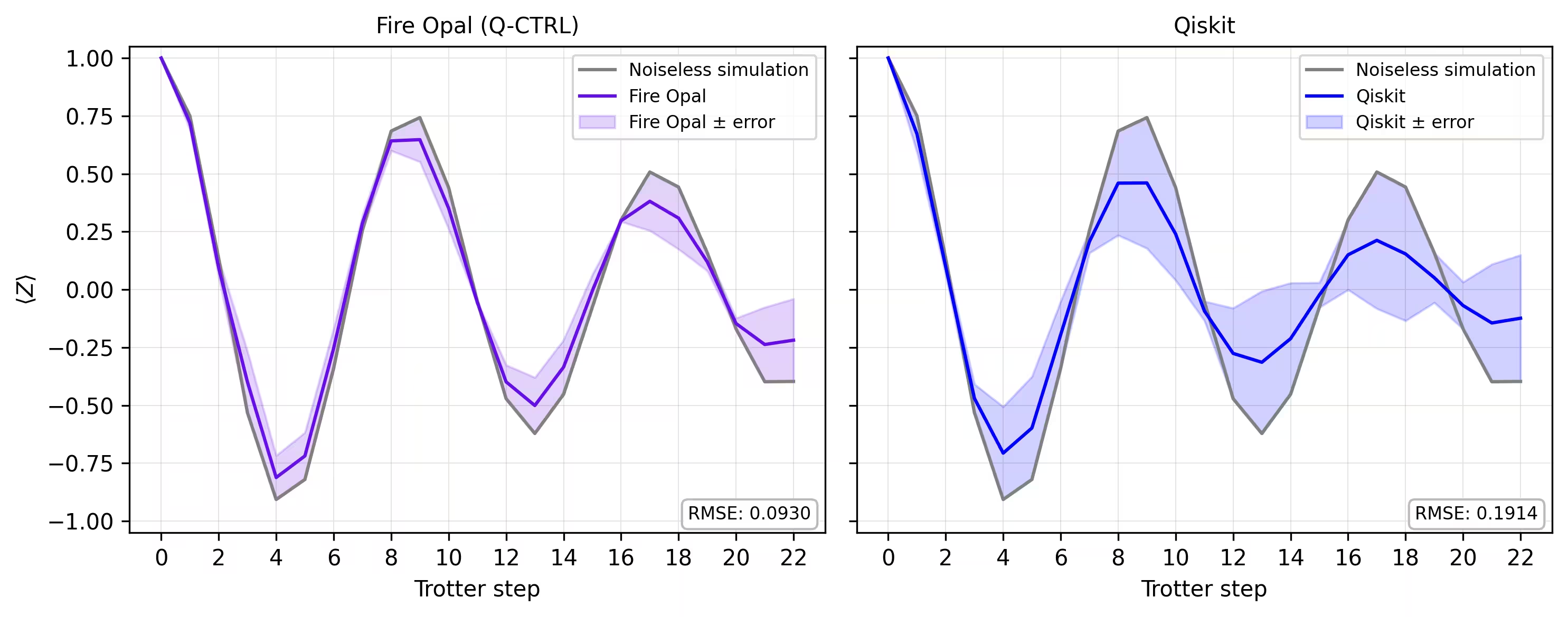
最後に、シミュレータから得られた磁化曲線と実際のハードウェアで得られた結果を比較します。両者を並べてプロットすることで、Fire Opal を使用したハードウェア実行がトロッターステップ全体にわたってノイズのないベースラインにどれほど一致するかを確認できます。
def make_correlators(test_counts, nq, d_ind_tot):
    mz = np.empty((nq, d_ind_tot))
    for d_ind in range(d_ind_tot):
        counts = test_counts[d_ind]
        for i in range(nq):
            mz[i, d_ind] = z_expectation(counts, i)
    average_z = np.mean(mz, axis=0)
    return np.concatenate((np.array([1]), average_z), axis=0)

sim_exp = make_correlators(sim_counts[0:22], nq=nq, d_ind_tot=22)
qiskit_exp = make_correlators(qiskit_counts[0:22], nq=nq, d_ind_tot=22)
qctrl_exp = [ev.data.evs for ev in result_qctrl[:]]
qctrl_exp_mean = np.concatenate(
    (np.array([1]), np.mean(qctrl_exp, axis=1)), axis=0
)
def make_expectations_plot(
    sim_z,
    depths,
    exp_qctrl=None,
    exp_qctrl_error=None,
    exp_qiskit=None,
    exp_qiskit_error=None,
    plot_from=0,
    plot_upto=23,
):
    import numpy as np
    import matplotlib.pyplot as plt

    depth_ticks = [0, 2, 4, 6, 8, 10, 12, 14, 16, 18, 20, 22]

    d = np.asarray(depths)[plot_from:plot_upto]
    sim = np.asarray(sim_z)[plot_from:plot_upto]

    qk = (
        None
        if exp_qiskit is None
        else np.asarray(exp_qiskit)[plot_from:plot_upto]
    )
    qc = (
        None
        if exp_qctrl is None
        else np.asarray(exp_qctrl)[plot_from:plot_upto]
    )

    qk_err = (
        None
        if exp_qiskit_error is None
        else np.asarray(exp_qiskit_error)[plot_from:plot_upto]
    )
    qc_err = (
        None
        if exp_qctrl_error is None
        else np.asarray(exp_qctrl_error)[plot_from:plot_upto]
    )

    # ---- helper(s) ----
    def rmse(a, b):
        if a is None or b is None:
            return None
        a = np.asarray(a, dtype=float)
        b = np.asarray(b, dtype=float)
        mask = np.isfinite(a) & np.isfinite(b)
        if not np.any(mask):
            return None
        diff = a[mask] - b[mask]
        return float(np.sqrt(np.mean(diff**2)))

    def plot_panel(ax, method_y, method_err, color, label, band_color=None):
        # Noiseless reference
        ax.plot(d, sim, color="grey", label="Noiseless simulation")

        # Method line + band
        if method_y is not None:
            ax.plot(d, method_y, color=color, label=label)
            if method_err is not None:
                lo = np.clip(method_y - method_err, -1.05, 1.05)
                hi = np.clip(method_y + method_err, -1.05, 1.05)
                ax.fill_between(
                    d,
                    lo,
                    hi,
                    alpha=0.18,
                    color=band_color if band_color else color,
                    label=f"{label} ± error",
                )
        else:
            ax.text(
                0.5,
                0.5,
                "No data",
                transform=ax.transAxes,
                ha="center",
                va="center",
                fontsize=10,
                color="0.4",
            )

        # RMSE box (vs sim)
        r = rmse(method_y, sim)
        if r is not None:
            ax.text(
                0.98,
                0.02,
                f"RMSE: {r:.4f}",
                transform=ax.transAxes,
                va="bottom",
                ha="right",
                fontsize=8,
                bbox=dict(
                    boxstyle="round,pad=0.35", fc="white", ec="0.7", alpha=0.9
                ),
            )
        # Axes
        ax.set_xticks(depth_ticks)
        ax.set_ylim(-1.05, 1.05)
        ax.grid(True, which="both", linewidth=0.4, alpha=0.4)
        ax.set_axisbelow(True)
        ax.legend(prop={"size": 8}, loc="best")

    fig, axes = plt.subplots(1, 2, figsize=(10, 4), dpi=300, sharey=True)

    axes[0].set_title("Fire Opal (Q-CTRL)", fontsize=10)
    plot_panel(
        axes[0],
        qc,
        qc_err,
        color="#680CE9",
        label="Fire Opal",
        band_color="#680CE9",
    )
    axes[0].set_xlabel("Trotter step")
    axes[0].set_ylabel(r"$\langle Z \rangle$")
    axes[1].set_title("Qiskit", fontsize=10)
    plot_panel(
        axes[1], qk, qk_err, color="blue", label="Qiskit", band_color="blue"
    )
    axes[1].set_xlabel("Trotter step")

    plt.tight_layout()
    plt.show()
depths = list(range(d_ind_tot + 1))
errors = np.abs(np.array(qctrl_exp_mean) - np.array(sim_exp))

errors_qiskit = np.abs(np.array(qiskit_exp) - np.array(sim_exp))
make_expectations_plot(
    sim_exp,
    depths,
    exp_qctrl=qctrl_exp_mean,
    exp_qctrl_error=errors,
    exp_qiskit=qiskit_exp,
    exp_qiskit_error=errors_qiskit,
)
参考文献
[1] Graph coloring. Wikipedia. Retrieved September 15, 2025, from https://en.wikipedia.org/wiki/Graph_coloring
チュートリアルアンケート
このチュートリアルについてのフィードバックをお寄せください。皆様のご意見は、コンテンツの改善およびユーザー体験の向上に役立てさせていただきます。
Note: This survey is provided by IBM Quantum and relates to the original English content. To give feedback on doQumentation's website, translations, or code execution, please open a GitHub issue.