Qiskit実装

このレッスンでは、量子もつれの応用レッスンで紹介したアイデアの一部をQiskitを使って実装します。

# Added by doQumentation — installs the packages this notebook needs if they are missing
import importlib.util

_needed = {"qiskit": "qiskit", "qiskit_aer": "qiskit-aer"}
_missing = [pip for module, pip in _needed.items()
            if importlib.util.find_spec(module) is None]
# One at a time, so a package that fails to install does not block the others
for _pip in _missing:
    %pip install -q {_pip}
if not _missing:
    print("\u2713 All required packages are installed")

from qiskit import __version__

print(__version__)

2.1.1

from qiskit import QuantumCircuit, QuantumRegister, ClassicalRegister
from qiskit_aer import AerSimulator
from qiskit.visualization import plot_histogram, array_to_latex
from qiskit.result import marginal_distribution
from qiskit.circuit.library import UGate
from math import pi
import random

テレポーテーションプロトコルの量子Circuit実装を以下に示します。

qubit = QuantumRegister(1, "Q")
ebit0 = QuantumRegister(1, "A")
ebit1 = QuantumRegister(1, "B")
a = ClassicalRegister(1, "a")
b = ClassicalRegister(1, "b")

protocol = QuantumCircuit(qubit, ebit0, ebit1, a, b)

# Prepare ebit used for teleportation
protocol.h(ebit0)
protocol.cx(ebit0, ebit1)
protocol.barrier()

# Alice's operations
protocol.cx(qubit, ebit0)
protocol.h(qubit)
protocol.barrier()

# Alice measures and sends classical bits to Bob
protocol.measure(ebit0, a)
protocol.measure(qubit, b)
protocol.barrier()

# Bob uses the classical bits to conditionally apply gates
with protocol.if_test((a, 1)):
    protocol.x(ebit1)
with protocol.if_test((b, 1)):
    protocol.z(ebit1)

display(protocol.draw(output="mpl"))

このCircuitでは、前のレッスンで扱っていないQiskitのいくつかの機能を使用しています。具体的には barrier 関数と if_test 関数です。 barrier 関数は視覚的な区切りを作ってCircuit図を読みやすくするとともに、実際のハードウェア上でCircuitを実行する際のコンパイル時に、Qiskitがバリアをまたいだ各種の簡略化・最適化を行うのを防ぎます。 if_test 関数は、古典ビットまたはレジスタの値に応じて条件付きで操作を適用します。

このCircuitはまず $(\mathsf{A},\mathsf{B})$ を $\vert \phi^+\rangle$ 状態に初期化し（これ自体はプロトコルの一部ではありません）、次にアリスの操作、その後測定、最後にボブの操作を行います。 プロトコルが正しく動作することを確認するために、$\mathsf{Q}$ の初期化された $\vert 0\rangle$ 状態にランダムに生成した1Qubit Gateを適用し、テレポートするランダムな量子状態ベクトルを得ます。プロトコル実行後にそのGateの逆演算（すなわち共役転置）を $\mathsf{B}$ に適用することで、状態が $\vert 0\rangle$ に戻ったかどうかを測定してテレポーテーションを検証できます。

まず、ランダムなユニタリ1Qubit Gateを選択します。

random_gate = UGate(
    theta=random.random() * 2 * pi,
    phi=random.random() * 2 * pi,
    lam=random.random() * 2 * pi,
)

display(array_to_latex(random_gate.to_matrix()))

$$\begin{bmatrix} 0.9897212158 & -0.0195080103 - 0.141673401 i \\ 0.0603319186 + 0.1296609988 i & -0.8319925233 + 0.5360378028 i \\ \end{bmatrix}$$

次に、新しいテスト用Circuitを作成します。このCircuitはまず $\mathsf{Q}$ にランダムなGateを適用し、テレポーテーションCircuitを実行し、最後にランダムなGateの逆演算をQubit $\mathsf{B}$ に適用して測定します。 結果は確実に $0$ になるはずです。

# Create a new circuit including the same bits and qubits used in the
# teleportation protocol.

test = QuantumCircuit(qubit, ebit0, ebit1, a, b)

# Start with the randomly selected gate on Q

test.append(random_gate, qubit)
test.barrier()

# Append the entire teleportation protocol from above.

test = test.compose(protocol)
test.barrier()

# Finally, apply the inverse of the random unitary to B and measure.

test.append(random_gate.inverse(), ebit1)
result = ClassicalRegister(1, "Result")
test.add_register(result)
test.measure(ebit1, result)

display(test.draw(output="mpl"))

では、このCircuitに対してAerシミュレーターを実行し、出力のヒストグラムをプロットしてみましょう。 3つの古典ビットすべての統計が表示されます。一番下（左端）のビットは常に $0$ となり、Qubit $\mathsf{Q}$ が $\mathsf{B}$ に正常にテレポートされたことを示します。一方、残りの2つのビットはほぼ一様に分布するはずです。

result = AerSimulator().run(test).result()
statistics = result.get_counts()
display(plot_histogram(statistics))

必要に応じて、テスト結果のQubitのみに絞って統計をフィルタリングすることもできます。

filtered_statistics = marginal_distribution(statistics, [2])
display(plot_histogram(filtered_statistics))

超高密度符号化

超高密度符号化（Superdense coding）は、ある意味でテレポーテーションと相補的な目的を達成するプロトコルです。 テレポーテーションが2古典ビットの通信を用いて1Qubitを送信できる（1 e-bitのもつれを消費して）のに対し、超高密度符号化では1Qubitの量子通信を用いて2古典ビットを送信できます（こちらも1 e-bitのもつれを消費して）。

より詳しく説明すると、送信者（アリス）と受信者（ボブ）が1 e-bitのもつれを共有しています。 レッスン内の規約に従い、アリスはQubit $\mathsf{A}$ を、ボブはQubit $\mathsf{B}$ を持ち、ペア $(\mathsf{A},\mathsf{B})$ は状態 $\vert\phi^+\rangle$ にあります。 アリスは $c$ と $d$ で表される2つの古典ビットをボブに送りたいと考えており、1つのQubitを送ることでこれを実現します。

この成果は、テレポーテーションが達成するものほど興味深くないと見なすこともできます。 当面の間、Qubitを送ることは古典ビットを送ることよりはるかに困難になると思われるため、e-bitのコストを払ってまで1Qubitの量子通信を2ビットの古典通信と交換することは、ほとんど割に合わないように思えます。 しかし、だからといって超高密度符号化が興味深くないということにはなりません。これは非常に興味深いプロトコルです。

レッスンのテーマに即して言えば、超高密度符号化が興味深い理由の一つは、もつれの具体的かつ（情報理論の文脈では）かなり印象的な利用例を示しているからです。 Holevoの定理として知られる量子情報理論の有名な定理によると、共有されたもつれ状態を使わない場合、1Qubitを送ることで送信できる古典情報量は1ビットを超えることができません。 （Holevoの定理はこれよりも一般的です。正確な表現は技術的であり説明が必要ですが、これはその一つの帰結です。） つまり、超高密度符号化により、共有もつれはQubitを送ることで伝達できる古典情報容量を実質的に2倍にすることができます。

プロトコル

次の量子Circuit図は超高密度符号化プロトコルを描写しています。

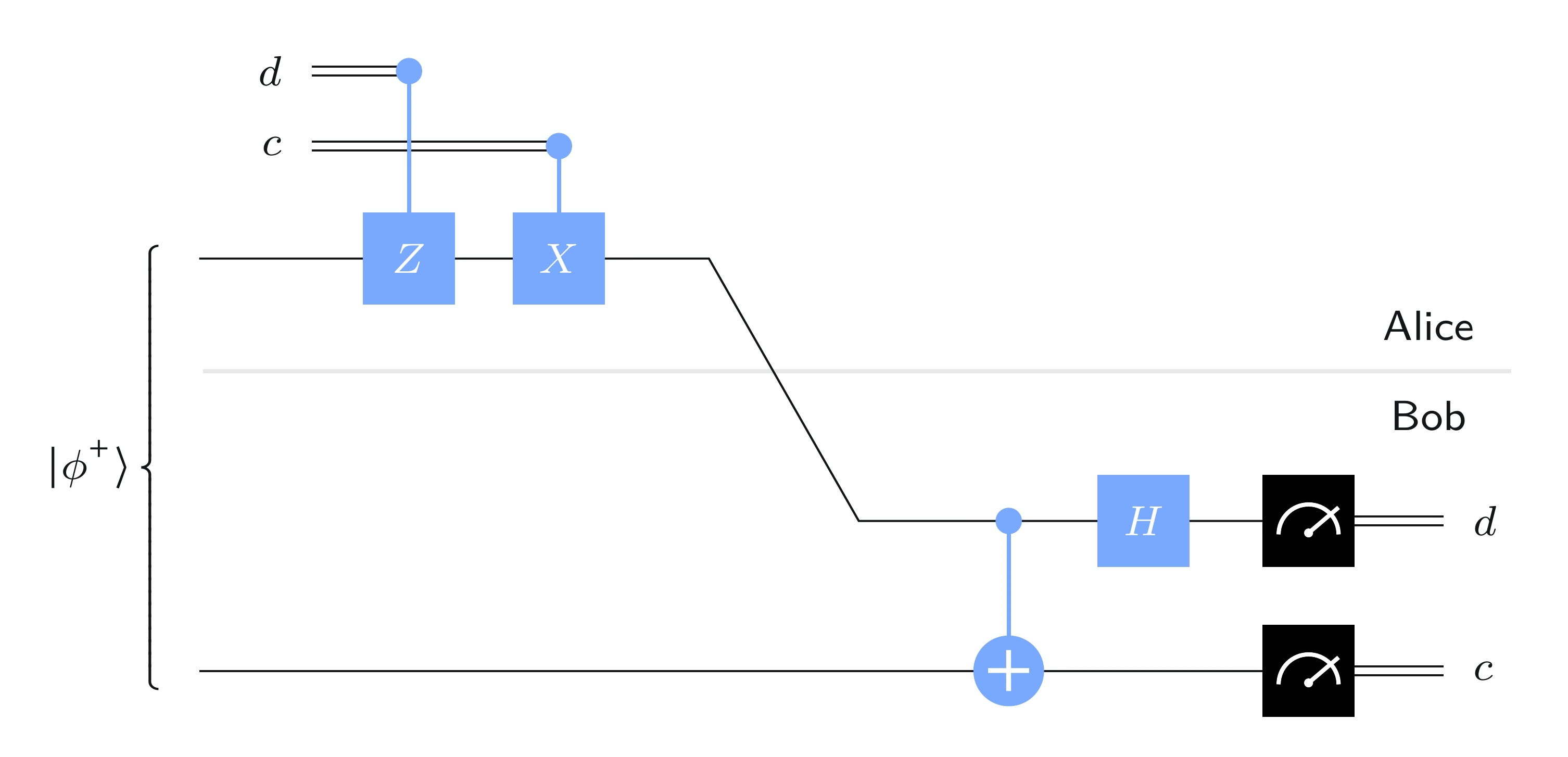
アリスの操作を言葉で説明すると以下の通りです。

1. $d=1$ の場合、アリスは自分のQubit $\mathsf{A}$ に $Z$ Gateを適用します（$d=0$ の場合は何もしません）。

2. $c=1$ の場合、アリスは自分のQubit $\mathsf{A}$ に $X$ Gateを適用します（$c=0$ の場合は何もしません）。

アリスはその後、自分のQubit $\mathsf{A}$ をボブに送ります。

ボブはQubit $\mathsf{A}$ を受け取ると、まず $\mathsf{A}$ を制御、$\mathsf{B}$ をターゲットとする制御NOTゲートを適用し、続いて $\mathsf{A}$ にアダマールゲートを適用します。 その後、$\mathsf{B}$ を測定して $c$ を、$\mathsf{A}$ を測定して $d$ を得ます。いずれも標準基底測定です。

解析

このプロトコルの考え方はシンプルです。 アリスはボブと共有したいベル状態を実質的に選択し、 自分のQubitをボブに送ります。ボブはどのベル状態をアリスが選んだかを測定で判定します。

つまり、はじめに $\vert\phi^+\rangle$ を共有している状態から、ビット $c$ と $d$ の値に応じて、アリスは自分のQubit $\mathsf{A}$ に $\mathbb{I}$、$X$、$Z$、または $XZ$ を適用することで、この状態をそのままにするか他のベル状態に変換します。

$$\begin{aligned} (\mathbb{I} \otimes \mathbb{I}) \vert \phi^+ \rangle & = \vert \phi^+\rangle \\ (\mathbb{I} \otimes Z) \vert \phi^+ \rangle & = \vert \phi^-\rangle \\ (\mathbb{I} \otimes X) \vert \phi^+ \rangle & = \vert \psi^+\rangle \\ (\mathbb{I} \otimes XZ) \vert \phi^+ \rangle & = \vert \psi^-\rangle \end{aligned}$$

ボブの操作は4つのベル状態に対して次の効果をもたらします。

$$\begin{aligned} \vert \phi^+\rangle & \mapsto \vert 00\rangle\\ \vert \phi^-\rangle & \mapsto \vert 01\rangle\\ \vert \psi^+\rangle & \mapsto \vert 10\rangle\\ \vert \psi^-\rangle & \mapsto -\vert 11\rangle\\ \end{aligned}$$

これは各状態に対してボブの操作の結果を直接計算することで確認できます。

したがって、ボブが測定を行うと、アリスがどのベル状態を選んだかを判定できます。 プロトコルが正しく動作することを確認するには、各ケースを個別に検証します。

• $cd = 00$ の場合、ボブが $\mathsf{A}$ を受け取った時点での $(\mathsf{B},\mathsf{A})$ の状態は $\vert \phi^+\rangle$ です。ボブはこの状態を $\vert 00\rangle$ に変換し、$cd = 00$ を得ます。

• $cd = 01$ の場合、ボブが $\mathsf{A}$ を受け取った時点での $(\mathsf{B},\mathsf{A})$ の状態は $\vert \phi^-\rangle$ です。ボブはこの状態を $\vert 01\rangle$ に変換し、$cd = 01$ を得ます。

• $cd = 10$ の場合、ボブが $\mathsf{A}$ を受け取った時点での $(\mathsf{B},\mathsf{A})$ の状態は $\vert \psi^+\rangle$ です。ボブはこの状態を $\vert 10\rangle$ に変換し、$cd = 10$ を得ます。

• $cd = 11$ の場合、ボブが $\mathsf{A}$ を受け取った時点での $(\mathsf{B},\mathsf{A})$ の状態は $\vert \psi^-\rangle$ です。ボブはこの状態を $-\vert 11\rangle$ に変換し、$cd = 11$ を得ます。（マイナス1の位相因子はここでは影響しません。）

超高密度符号化の実装

以下は超高密度符号化の簡単な実装です。送信するビットに応じてCircuitを構成します。まず送信する2ビットを選択します（後ほどランダムに選びますが、ここではとりあえず任意の値を設定します）。

c = "1"
d = "0"

次に、それに応じてCircuitを構築します。ここではQiskitのデフォルト名をQubitに使用します。上のQubitが $\mathsf{q}_0$、下のQubitが $\mathsf{q}_1$ となります。

protocol = QuantumCircuit(2)

# Prepare ebit used for superdense coding
protocol.h(0)
protocol.cx(0, 1)
protocol.barrier()

# Alice's operations
if d == "1":
    protocol.z(0)
if c == "1":
    protocol.x(0)
protocol.barrier()

# Bob's actions
protocol.cx(0, 1)
protocol.h(0)
protocol.measure_all()

display(protocol.draw(output="mpl"))

新しい点としては measure_all 関数があります。これはすべてのQubitを測定し、結果を1つの古典レジスタに格納します（この場合は2ビットになります）。

Aerシミュレーターを実行すると、期待通りの出力が得られます。

result = AerSimulator().run(protocol).result()
statistics = result.get_counts()

for outcome, frequency in statistics.items():
    print(f"Measured {outcome} with frequency {frequency}")

display(plot_histogram(statistics))

Measured 10 with frequency 1024

次に、追加のQubitをランダムビット生成器として使用しましょう。本質的には公平なコインを投げることに相当します。これを使って $c$ と $d$ をランダムに選択し、超高密度符号化プロトコルを実行します。

rbg = QuantumRegister(1, "coin")
ebit0 = QuantumRegister(1, "A")
ebit1 = QuantumRegister(1, "B")

Alice_c = ClassicalRegister(1, "Alice c")
Alice_d = ClassicalRegister(1, "Alice d")

test = QuantumCircuit(rbg, ebit0, ebit1, Alice_d, Alice_c)

# Initialize the ebit
test.h(ebit0)
test.cx(ebit0, ebit1)
test.barrier()

# Use the 'coin' qubit twice to generate Alice's bits c and d.
test.h(rbg)
test.measure(rbg, Alice_c)
test.h(rbg)
test.measure(rbg, Alice_d)
test.barrier()

# Now the protocol runs, starting with Alice's actions, which depend
# on her bits.
with test.if_test((Alice_d, 1), label="Z"):
    test.z(ebit0)
with test.if_test((Alice_c, 1), label="X"):
    test.x(ebit0)
test.barrier()

# Bob's actions
test.cx(ebit0, ebit1)
test.h(ebit0)
test.barrier()

Bob_c = ClassicalRegister(1, "Bob c")
Bob_d = ClassicalRegister(1, "Bob d")
test.add_register(Bob_d)
test.add_register(Bob_c)
test.measure(ebit0, Bob_d)
test.measure(ebit1, Bob_c)

display(test.draw(output="mpl"))

Aerシミュレーターを実行すると、アリスとボブの古典ビットが常に一致していることが確認できます。

result = AerSimulator().run(test).result()
statistics = result.get_counts()
display(plot_histogram(statistics))

Qiskitによる実装

CHSHゲームと上記で定義した量子戦略をQiskitで次のように実装できます。

まず、ゲーム自体の定義です。任意の戦略を引数として渡せるようになっています。

def chsh_game(strategy):
    # This function runs the CHSH game, using the strategy (a function
    # from two bits to two bits), returning 1 for a win and 0 for a loss.

    # Choose x and y randomly
    x, y = random.randint(0, 1), random.randint(0, 1)

    # Use the strategy to determine a and b
    a, b = strategy(x, y)

    # Decide if the strategy wins or loses
    if (a != b) == (x & y):
        return 1  # Win
    return 0  # Lose

次に、アリスとボブへの質問に応じたCircuitを出力する関数を作成します。簡単のためQubitにはデフォルトの名前を使い、アリスとボブの操作には組み込みの $R_y(\theta)$ ゲートを使用します。

def chsh_circuit(x, y):
    # This function creates a `QuantumCircuit` implementing the quantum
    # strategy described above (including the e-bit preparation).

    qc = QuantumCircuit(2, 2)

    # Prepare an e-bit
    qc.h(0)
    qc.cx(0, 1)
    qc.barrier()

    # Alice's actions
    if x == 0:
        qc.ry(0, 0)
    else:
        qc.ry(-pi / 2, 0)
    qc.measure(0, 0)

    # Bob's actions
    if y == 0:
        qc.ry(-pi / 4, 1)
    else:
        qc.ry(pi / 4, 1)
    qc.measure(1, 1)

    return qc

以下は、質問の組み合わせに応じた4つの可能なCircuitです。

# Draw the four possible circuits

print("(x,y) = (0,0)")
display(chsh_circuit(0, 0).draw(output="mpl"))

print("(x,y) = (0,1)")
display(chsh_circuit(0, 1).draw(output="mpl"))

print("(x,y) = (1,0)")
display(chsh_circuit(1, 0).draw(output="mpl"))

print("(x,y) = (1,1)")
display(chsh_circuit(1, 1).draw(output="mpl"))

(x,y) = (0,0)

(x,y) = (0,1)

(x,y) = (1,0)

(x,y) = (1,1)

次に、Aerシミュレーターを使用して、与えられた入力のペア $(x,y)$ に対してCircuitを1回実行するジョブを作成します。

def quantum_strategy(x, y):
    # This function runs the appropriate quantum circuit defined above
    # one time and returns the measurement results

    # Setting `shots=1` to run the circuit once
    result = AerSimulator().run(chsh_circuit(x, y), shots=1).result()
    statistics = result.get_counts()

    # Determine the output bits and return them
    bits = list(statistics.keys())[0]
    a, b = bits[0], bits[1]
    return a, b

最後に、ゲームを1000回プレイして、この戦略の勝率を計算します。

NUM_GAMES = 1000
TOTAL_SCORE = 0

for _ in range(NUM_GAMES):
    TOTAL_SCORE += chsh_game(quantum_strategy)

print("Fraction of games won:", TOTAL_SCORE / NUM_GAMES)

Fraction of games won: 0.867

古典的な戦略も定義して、その性能を確認してみましょう。 これは数ある戦略の一例に過ぎませんが、コードを変更すれば他の戦略もテストできます。なお、これは最適な古典的戦略のひとつです。

def classical_strategy(x, y):
    # This function implements just one example of an optimal classical
    # strategy for the CHSH game. Other classical strategies can be
    # implemented by changing the bit values assigned to a and b.

    # Alice's answer
    if x == 0:
        a = 0
    elif x == 1:
        a = 1

    # Bob's answer
    if y == 0:
        b = 1
    elif y == 1:
        b = 0

    return a, b

こちらもゲームを1000回プレイして、勝率を確認してみましょう。

NUM_GAMES = 1000
TOTAL_SCORE = 0

for _ in range(NUM_GAMES):
    TOTAL_SCORE += chsh_game(classical_strategy)

print("Fraction of games won:", TOTAL_SCORE / NUM_GAMES)

Fraction of games won: 0.747

ランダム性が伴うものの、1000回の試行後に統計が大きくずれる可能性はほとんどありません。量子戦略は約85%の確率で勝利する一方、古典的な戦略では約75%を超えることができません。