量子シミュレーション

備考

Yukio Kawashima（2024年5月30日）

元の講義の PDF をダウンロード できます。コードスニペットは静的画像であるため、一部が非推奨になっている場合があります。

この実験を実行するおおよその QPU 時間は 7 秒です。

（このノートブックは、Qiskit Algorithms の現在は非推奨となったチュートリアルノートブックをもとにしています。）

1. はじめに

実時間発展の手法として、トロッタリゼーション（Trotterization）は、あるタイムスライスにおけるシステムの時間発展を近似するように選ばれた量子ゲートを繰り返し適用することで構成されます。シュレーディンガー方程式から、時刻 $t=0$ に状態 $\vert\psi(0)\rangle$ にあるシステムの時間発展は次の形で表されます：

$$\vert \psi(t) \rangle = e^{-i H t} \vert \psi(0) \rangle \text{,}$$

ここで $H$ はシステムを支配する時間非依存なハミルトニアンです。$H=\sum_j a_j P_j$ と書けるハミルトニアンを考えます。$P_j$ は $n$ 個の Qubit に作用するパウリ項のテンソル積を表します。これらのパウリ項は互いに交換する場合もあれば、しない場合もあります。$t=0$ における状態が与えられたとき、量子コンピュータを用いて、後の時刻における状態 $|\psi(t)\rangle$ をどのように求めればよいでしょうか？演算子の指数関数はテイラー展開を通じて理解できます：

$$e^{-i H t} = 1-iHt-\frac{1}{2}H^2t^2+...$$

$e^{iZ}$ のような非常に基本的な指数関数は、コンパクトな量子ゲートのセットを用いて量子コンピュータ上で簡単に実装できます。ほとんどの興味深いハミルトニアンは単一の項だけではなく、多数の項を持ちます。$H = H_1+H_2$ の場合に何が起こるか見てみましょう：

$$e^{-i H t} = 1-i(H_1+H_2)t-\frac{1}{2}(H_1+H_2)^2t^2+...$$

$H_1$ と $H_2$ が交換する場合、次のよく知られた式が成り立ちます（数値や変数 $a$, $b$ でも同様です）：

$$e^{-i (a+b) t} = e^{-i a t}e^{-i b t}$$

しかし、演算子が交換しない場合、テイラー展開の項を並べ替えてこのように簡略化することはできません。そのため、複雑なハミルトニアンを量子ゲートで表現することは難しい課題となります。

一つの解決策は、時間 $t$ を非常に小さく取ることで、テイラー展開の一次項が支配的になるようにすることです。その仮定のもとで：

$$e^{-i (H_1+H_2) t} \approx 1-i(H_1+H_2)t \approx (1-i H_1 t)(1-i H_2 t) \approx e^{-i H_1 t}e^{-i H_2 t}$$

もちろん、より長い時間だけ状態を発展させる必要がある場合もあります。それには、このような小さな時間ステップを多数繰り返すことで実現します。このプロセスをトロッタリゼーションと呼びます：

$$\vert \psi(t) \rangle \approx \left(\prod_j e^{-i a_j P_j t/r} \right)^r \vert\psi(0) \rangle \text{,}$$

ここで $t/r$ は選択するタイムスライス（発展ステップ）です。その結果、$r$ 回適用するゲートが作成されます。タイムステップが小さいほど近似精度は高まりますが、同時に Circuit が深くなり、実際には誤差の蓄積が増大します（近代の量子デバイスでは無視できない問題です）。

今回は、$N=2$ および $N=6$ サイトの線形格子上のイジングモデルの時間発展を調べます。これらの格子は、最近接のスピン $\sigma_i$ どうしのみが相互作用するスピン配列から成ります。各スピンは $\uparrow$ と $\downarrow$ の二方向を取り得、それぞれ磁化 $+1$ と $-1$ に対応します。

$$H = - J \sum_{i=0}^{N-2} Z_i Z_{i+1} - h \sum_{i=0}^{N-1} X_i \text{,}$$

ここで $J$ は相互作用エネルギーを、$h$ は外部磁場の大きさ（上式では x 方向ですが、後で変更します）を表します。パウリ行列を用いてこの式を書き直し、外部磁場が横方向に対して角度 $\alpha$ をなすとすると、

$$H = -J \sum_{i=0}^{N-2} Z_i Z_{i+1} -h \sum_{i=0}^{N-1} (\sin\alpha Z_i + \cos\alpha X_i) \text{.}$$

このハミルトニアンは外部磁場の効果を容易に研究できる点で有用です。計算基底では、系は以下のようにエンコードされます：

量子状態	スピン表現
$\lvert 0 0 0 0 \rangle$	$\uparrow\uparrow\uparrow\uparrow$
$\lvert 1 0 0 0 \rangle$	$\downarrow\uparrow\uparrow\uparrow$
$\ldots$	$\ldots$
$\lvert 1 1 1 1 \rangle$	$\downarrow\downarrow\downarrow\downarrow$

それでは、このような量子系の時間発展を調べていきます。特に、磁化などのシステムの特定の物理量の時間発展を可視化します。

1.1 必要条件

このチュートリアルを開始する前に、以下のパッケージがインストールされていることを確認してください：

• Qiskit SDK v1.2 以降 （ pip install qiskit ）
• Qiskit Runtime v0.30 以降 （ pip install qiskit-ibm-runtime ）
• Numpy v1.24.1 以降 < 2 （ pip install numpy ）

1.2 ライブラリのインポート

MatrixExponential や QDrift など有用なライブラリも含まれていますが、このノートブックでは使用しません。時間があればぜひ試してみてください！

# Added by doQumentation — required packages for this notebook
!pip install -q matplotlib numpy qiskit qiskit-ibm-runtime

# Check the version of Qiskit
import qiskit

qiskit.__version__

'2.0.2'

# Import the qiskit library
import numpy as np
import matplotlib.pylab as plt
import warnings

from qiskit import QuantumCircuit
from qiskit.circuit.library import PauliEvolutionGate
from qiskit.primitives import StatevectorEstimator
from qiskit.quantum_info import Statevector, SparsePauliOp
from qiskit.synthesis import (
    SuzukiTrotter,
    LieTrotter,
)
from qiskit.transpiler.preset_passmanagers import generate_preset_pass_manager

from qiskit_ibm_runtime import QiskitRuntimeService, SamplerV2

warnings.filterwarnings("ignore")

2. 問題のマッピング

2.1 横磁場イジングハミルトニアンの定義

ここでは 1 次元横磁場イジングモデルを考えます。

まず、システムパラメータ $N$、$J$、$h$、$\alpha$ を受け取り、ハミルトニアンを SparsePauliOp として返す関数を作成します。SparsePauliOp は、重み付きパウリ項を用いた演算子のスパース表現です。

def get_hamiltonian(nqubits, J, h, alpha):
    # List of Hamiltonian terms as 3-tuples containing
    # (1) the Pauli string,
    # (2) the qubit indices corresponding to the Pauli string,
    # (3) the coefficient.
    ZZ_tuples = [("ZZ", [i, i + 1], -J) for i in range(0, nqubits - 1)]
    Z_tuples = [("Z", [i], -h * np.sin(alpha)) for i in range(0, nqubits)]
    X_tuples = [("X", [i], -h * np.cos(alpha)) for i in range(0, nqubits)]

    # We create the Hamiltonian as a SparsePauliOp, via the method
    # `from_sparse_list`, and multiply by the interaction term.
    hamiltonian = SparsePauliOp.from_sparse_list(
        [*ZZ_tuples, *Z_tuples, *X_tuples], num_qubits=nqubits
    )
    return hamiltonian.simplify()

ハミルトニアンの定義

ここでは例として、サイズ $N=6$、$J=0.2$、$h=1.2$、$\alpha=\frac{\pi}{8.0}$ のシステムを考えます。

n_qubits = 6

hamiltonian = get_hamiltonian(nqubits=n_qubits, J=0.2, h=1.2, alpha=np.pi / 8.0)
hamiltonian

SparsePauliOp(['IIIIZZ', 'IIIZZI', 'IIZZII', 'IZZIII', 'ZZIIII', 'IIIIIZ', 'IIIIZI', 'IIIZII', 'IIZIII', 'IZIIII', 'ZIIIII', 'IIIIIX', 'IIIIXI', 'IIIXII', 'IIXIII', 'IXIIII', 'XIIIII'],
              coeffs=[-0.2       +0.j, -0.2       +0.j, -0.2       +0.j, -0.2       +0.j,
 -0.2       +0.j, -0.45922012+0.j, -0.45922012+0.j, -0.45922012+0.j,
 -0.45922012+0.j, -0.45922012+0.j, -0.45922012+0.j, -1.10865544+0.j,
 -1.10865544+0.j, -1.10865544+0.j, -1.10865544+0.j, -1.10865544+0.j,
 -1.10865544+0.j])

2.2 時間発展シミュレーションのパラメータ設定

ここでは、3 種類のトロッタリゼーション手法を考えます：

• Lie–Trotter（一次）
• 二次 Suzuki–Trotter
• 四次 Suzuki–Trotter

後の二つは演習と付録で使用します。

num_timesteps = 60
evolution_time = 30.0
dt = evolution_time / num_timesteps
product_formula_lt = LieTrotter()
product_formula_st2 = SuzukiTrotter(order=2)
product_formula_st4 = SuzukiTrotter(order=4)

2.3 量子 Circuit の準備 1（初期状態）

初期状態を作成します。ここでは $\uparrow\uparrow\downarrow\downarrow\uparrow\uparrow$ のスピン配置から始めます。

initial_circuit = QuantumCircuit(n_qubits)
initial_circuit.prepare_state("001100")
# Change reps and see the difference when you decompose the circuit
initial_circuit.decompose(reps=1).draw("mpl")

2.4 量子 Circuit の準備 2（時間発展の単一 Circuit）

ここでは Lie–Trotter を用いて、単一タイムステップの Circuit を構築します。

Lie 積公式（一次）は LieTrotter クラスで実装されています。一次公式は、はじめに述べた近似から成り、和の行列指数関数を行列指数関数の積で近似します：

$$e^{H_1+H_2} \approx e^{H_1} e^{H_2}$$

前述のとおり、非常に深い Circuit は誤差の蓄積を招き、現代の量子コンピュータにとって問題となります。2 Qubit ゲートは 1 Qubit ゲートよりもエラー率が高いため、特に注目すべき指標は 2 Qubit Circuit の深さです。実際に重要なのはトランスパイル後の 2 Qubit Circuit の深さです（量子コンピュータが実際に実行するのはそのCircuitだからです）。しかし、今はシミュレータを使う段階でも、この Circuit の演算数を数える習慣をつけておきましょう。

single_step_evolution_gates_lt = PauliEvolutionGate(
    hamiltonian, dt, synthesis=product_formula_lt
)
single_step_evolution_lt = QuantumCircuit(n_qubits)
single_step_evolution_lt.append(
    single_step_evolution_gates_lt, single_step_evolution_lt.qubits
)

print(
    f"""
Trotter step with Lie-Trotter
-----------------------------
Depth: {single_step_evolution_lt.decompose(reps=3).depth()}
Gate count: {len(single_step_evolution_lt.decompose(reps=3))}
Nonlocal gate count: {single_step_evolution_lt.decompose(reps=3).num_nonlocal_gates()}
Gate breakdown: {", ".join([f"{k.upper()}: {v}" for k, v in single_step_evolution_lt.decompose(reps=3).count_ops().items()])}
"""
)
single_step_evolution_lt.decompose(reps=3).draw("mpl", fold=-1)

Trotter step with Lie-Trotter
-----------------------------
Depth: 17
Gate count: 27
Nonlocal gate count: 10
Gate breakdown: U3: 12, CX: 10, U1: 5

2.5 測定する演算子の設定

磁化演算子 $\sum_i \langle Z_i \rangle / N$ と 平均スピン相関演算子 $\sum_i \langle Z_i Z_{i+1} \rangle/ (N - 1)$ を定義します。

magnetization = (
    SparsePauliOp.from_sparse_list(
        [("Z", [i], 1.0) for i in range(0, n_qubits)], num_qubits=n_qubits
    )
    / n_qubits
)
correlation = SparsePauliOp.from_sparse_list(
    [("ZZ", [i, i + 1], 1.0) for i in range(0, n_qubits - 1)], num_qubits=n_qubits
) / (n_qubits - 1)
print("magnetization : ", magnetization)
print("correlation : ", correlation)

magnetization :  SparsePauliOp(['IIIIIZ', 'IIIIZI', 'IIIZII', 'IIZIII', 'IZIIII', 'ZIIIII'],
              coeffs=[0.16666667+0.j, 0.16666667+0.j, 0.16666667+0.j, 0.16666667+0.j,
 0.16666667+0.j, 0.16666667+0.j])
correlation :  SparsePauliOp(['IIIIZZ', 'IIIZZI', 'IIZZII', 'IZZIII', 'ZZIIII'],
              coeffs=[0.2+0.j, 0.2+0.j, 0.2+0.j, 0.2+0.j, 0.2+0.j])

2.6 時間発展シミュレーションの実行

エネルギー（ハミルトニアンの期待値）、磁化（磁化演算子の期待値）、平均スピン相関（平均スピン相関演算子の期待値）を観測します。Qiskit の StatevectorEstimator（EstimatorV2）プリミティブは、オブザーバブルの期待値 $\langle\psi\vert\hat{O}\vert\psi\rangle$ を推定します。

# Initiate the circuit
evolved_state = QuantumCircuit(initial_circuit.num_qubits)
# Start from the initial spin configuration
evolved_state.append(initial_circuit, evolved_state.qubits)
# Initiate Estimator (V2)
estimator = StatevectorEstimator()
# Set number of shots
shots = 10000
# Translate the precision required from the number of shots
precision = np.sqrt(1 / shots)
energy_list = []
mag_list = []
corr_list = []
# Estimate expectation values for t=0.0
job = estimator.run(
    [(evolved_state, [hamiltonian, magnetization, correlation])], precision=precision
)
# Get estimated expectation values
evs = job.result()[0].data.evs
energy_list.append(evs[0])
mag_list.append(evs[1])
corr_list.append(evs[2])
# Start time evolution
for n in range(num_timesteps):
    # Expand the circuit to describe delta-t
    evolved_state.append(single_step_evolution_gates_lt, evolved_state.qubits)
    # Estimate expectation values at delta-t
    job = estimator.run(
        [(evolved_state, [hamiltonian, magnetization, correlation])],
        precision=precision,
    )
    # Retrieve results (expectation values)
    evs = job.result()[0].data.evs
    energy_list.append(evs[0])
    mag_list.append(evs[1])
    corr_list.append(evs[2])
# Transform the list of expectation values (at each time step) to arrays
energy_array = np.array(energy_list)
mag_array = np.array(mag_list)
corr_array = np.array(corr_list)

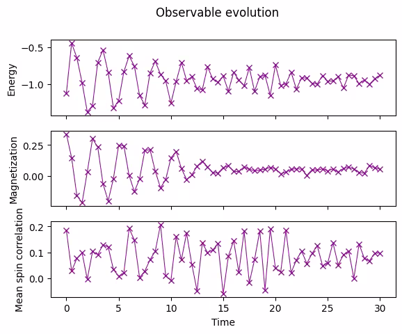
2.7 観測量の時間発展をプロットする

測定した期待値を時間に対してプロットします。

fig, axes = plt.subplots(3, sharex=True)
times = np.linspace(0, evolution_time, num_timesteps + 1)  # includes initial state
axes[0].plot(
    times,
    energy_array,
    label="First order",
    marker="x",
    c="darkmagenta",
    ls="-",
    lw=0.8,
)
axes[1].plot(
    times, mag_array, label="First order", marker="x", c="darkmagenta", ls="-", lw=0.8
)
axes[2].plot(
    times, corr_array, label="First order", marker="x", c="darkmagenta", ls="-", lw=0.8
)
axes[0].set_ylabel("Energy")
axes[1].set_ylabel("Magnetization")
axes[2].set_ylabel("Mean spin correlation")
axes[2].set_xlabel("Time")
fig.suptitle("Observable evolution")

Text(0.5, 0.98, 'Observable evolution')

3. 演習1：2次鈴木–トロッター法によるシミュレーションの実行

上で示したLie–Trotter法の例にならい、2次鈴木–トロッター法によるシミュレーションを試してみましょう。

2次鈴木–トロッター法はQiskitのSuzukiTrotterクラスを使って利用できます。この公式を使うと、2次分解は次のようになります：

$$e^{H_1+H_2} \approx e^{H_1/2}e^{H_2}e^{H_1/2}$$

3.1 1タイムステップ分の回路を構成する

product_formula_st2（SuzukiTrotter(order=2)）を使い、2次鈴木–トロッター法で1タイムステップ分の回路を構成してください。また、ゲート数と回路の深さを数え、Lie–Trotter法と比較してください。

# Modify the line below (Use PauliEvolutionGate)
single_step_evolution_gates_st2 = PauliEvolutionGate(
    hamiltonian, dt, synthesis=product_formula_st2
)
single_step_evolution_st2 = QuantumCircuit(n_qubits)
single_step_evolution_st2.append(
    single_step_evolution_gates_st2, single_step_evolution_st2.qubits
)
# Let us print some stats
print(
    f"""
Trotter step with second-order Suzuki-Trotter
-----------------------------
Depth: {single_step_evolution_st2.decompose(reps=3).depth()}
Gate count: {len(single_step_evolution_st2.decompose(reps=3))}
Nonlocal gate count: {single_step_evolution_st2.decompose(reps=3).num_nonlocal_gates()}
Gate breakdown: {", ".join([f"{k.upper()}: {v}" for k, v in single_step_evolution_st2.decompose(reps=3).count_ops().items()])}
"""
)
single_step_evolution_st2.decompose(reps=2).draw("mpl", fold=-1)

Trotter step with second-order Suzuki-Trotter
-----------------------------
Depth: 34
Gate count: 53
Nonlocal gate count: 20
Gate breakdown: U3: 23, CX: 20, U1: 10

3.2 時間発展シミュレーションを実行する

2次鈴木–トロッター法を使って時間発展を実行します。

# Initiate the circuit
evolved_state = QuantumCircuit(initial_circuit.num_qubits)
# Start from the initial spin configuration
evolved_state.append(initial_circuit, evolved_state.qubits)
# Initiate Estimator (V2)
estimator = StatevectorEstimator()
# Set number of shots
shots = 10000
# Translate the precision required from the number of shots
precision = np.sqrt(1 / shots)
energy_list_st2 = []
mag_list_st2 = []
corr_list_st2 = []
# Estimate expectation values for t=0.0
job = estimator.run(
    [(evolved_state, [hamiltonian, magnetization, correlation])], precision=precision
)
# Get estimated expectation values
evs = job.result()[0].data.evs
energy_list_st2.append(evs[0])
mag_list_st2.append(evs[1])
corr_list_st2.append(evs[2])
# Start time evolution
for n in range(num_timesteps):
    # Expand the circuit to describe delta-t
    evolved_state.append(single_step_evolution_gates_st2, evolved_state.qubits)
    # Estimate expectation values at delta-t
    job = estimator.run(
        [(evolved_state, [hamiltonian, magnetization, correlation])],
        precision=precision,
    )
    # Retrieve results (expectation values)
    evs = job.result()[0].data.evs
    energy_list_st2.append(evs[0])
    mag_list_st2.append(evs[1])
    corr_list_st2.append(evs[2])
# Transform the list of expectation values (at each time step) to arrays
energy_array_st2 = np.array(energy_list_st2)
mag_array_st2 = np.array(mag_list_st2)
corr_array_st2 = np.array(corr_list_st2)

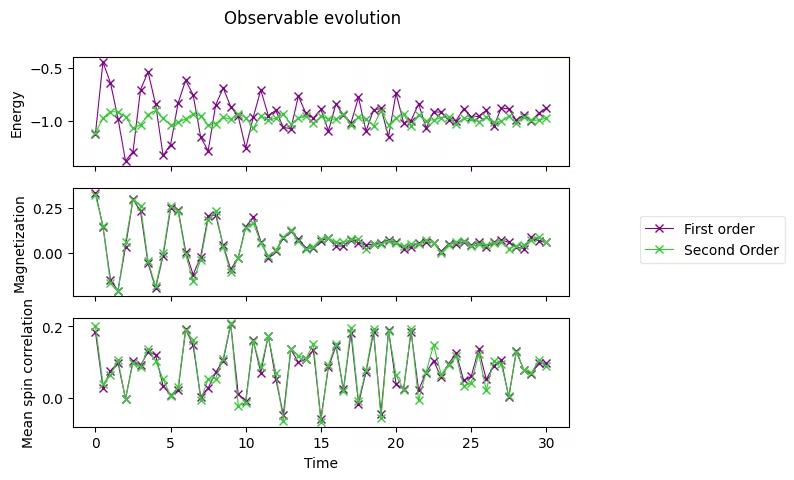
3.3 2次鈴木–トロッター法の結果をプロットする

axes[0].plot(
    times,
    energy_array_st2,
    label="Second Order",
    marker="x",
    c="limegreen",
    ls="-",
    lw=0.8,
)
axes[1].plot(
    times,
    mag_array_st2,
    label="Second Order",
    marker="x",
    c="limegreen",
    ls="-",
    lw=0.8,
)
axes[2].plot(
    times,
    corr_array_st2,
    label="Second Order",
    marker="x",
    c="limegreen",
    ls="-",
    lw=0.8,
)

# Replace the legend
# legend.remove()
legend = fig.legend(
    *axes[0].get_legend_handles_labels(),
    bbox_to_anchor=(1.0, 0.5),
    loc="center left",
    framealpha=0.5,
)
fig

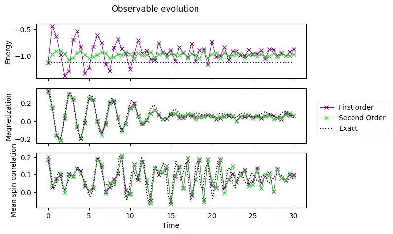
3.4 厳密解と比較する

以下のデータは、古典コンピュータであらかじめ計算した厳密解です。

exact_times = np.array(
    [
        0.0,
        0.3,
        0.6,
        0.8999999999999999,
        1.2,
        1.5,
        1.7999999999999998,
        2.1,
        2.4,
        2.6999999999999997,
        3.0,
        3.3,
        3.5999999999999996,
        3.9,
        4.2,
        4.5,
        4.8,
        5.1,
        5.3999999999999995,
        5.7,
        6.0,
        6.3,
        6.6,
        6.8999999999999995,
        7.199999999999999,
        7.5,
        7.8,
        8.1,
        8.4,
        8.7,
        9.0,
        9.299999999999999,
        9.6,
        9.9,
        10.2,
        10.5,
        10.799999999999999,
        11.1,
        11.4,
        11.7,
        12.0,
        12.299999999999999,
        12.6,
        12.9,
        13.2,
        13.5,
        13.799999999999999,
        14.1,
        14.399999999999999,
        14.7,
        15.0,
        15.299999999999999,
        15.6,
        15.899999999999999,
        16.2,
        16.5,
        16.8,
        17.099999999999998,
        17.4,
        17.7,
        18.0,
        18.3,
        18.599999999999998,
        18.9,
        19.2,
        19.5,
        19.8,
        20.099999999999998,
        20.4,
        20.7,
        21.0,
        21.3,
        21.599999999999998,
        21.9,
        22.2,
        22.5,
        22.8,
        23.099999999999998,
        23.4,
        23.7,
        24.0,
        24.3,
        24.599999999999998,
        24.9,
        25.2,
        25.5,
        25.8,
        26.099999999999998,
        26.4,
        26.7,
        27.0,
        27.3,
        27.599999999999998,
        27.9,
        28.2,
        28.5,
        28.799999999999997,
        29.099999999999998,
        29.4,
        29.7,
        30.0,
    ]
)
exact_energy = np.array(
    [
        -1.1184402376762155,
        -1.1184402376762157,
        -1.1184402376762157,
        -1.1184402376762148,
        -1.1184402376762153,
        -1.1184402376762155,
        -1.1184402376762148,
        -1.118440237676216,
        -1.118440237676216,
        -1.1184402376762166,
        -1.1184402376762148,
        -1.118440237676216,
        -1.1184402376762153,
        -1.1184402376762148,
        -1.118440237676217,
        -1.118440237676215,
        -1.1184402376762161,
        -1.1184402376762157,
        -1.118440237676217,
        -1.1184402376762161,
        -1.1184402376762137,
        -1.1184402376762161,
        -1.1184402376762161,
        -1.118440237676218,
        -1.1184402376762155,
        -1.1184402376762166,
        -1.1184402376762155,
        -1.1184402376762137,
        -1.1184402376762186,
        -1.1184402376762215,
        -1.1184402376762148,
        -1.118440237676216,
        -1.1184402376762166,
        -1.1184402376762148,
        -1.1184402376762121,
        -1.1184402376762166,
        -1.1184402376762181,
        -1.1184402376762137,
        -1.1184402376762148,
        -1.1184402376762193,
        -1.1184402376762108,
        -1.1184402376762144,
        -1.118440237676217,
        -1.1184402376762197,
        -1.1184402376762153,
        -1.1184402376762161,
        -1.1184402376762184,
        -1.1184402376762126,
        -1.118440237676214,
        -1.118440237676214,
        -1.1184402376762161,
        -1.118440237676212,
        -1.1184402376762164,
        -1.118440237676217,
        -1.1184402376762121,
        -1.1184402376762157,
        -1.1184402376762212,
        -1.1184402376762217,
        -1.1184402376762206,
        -1.118440237676222,
        -1.1184402376762166,
        -1.118440237676212,
        -1.1184402376762137,
        -1.11844023767622,
        -1.1184402376762206,
        -1.118440237676219,
        -1.1184402376762153,
        -1.1184402376762164,
        -1.118440237676209,
        -1.1184402376762144,
        -1.1184402376762161,
        -1.118440237676216,
        -1.1184402376762173,
        -1.118440237676214,
        -1.1184402376762093,
        -1.1184402376762184,
        -1.1184402376762126,
        -1.118440237676213,
        -1.1184402376762195,
        -1.1184402376762095,
        -1.1184402376762075,
        -1.1184402376762197,
        -1.1184402376762141,
        -1.1184402376762146,
        -1.1184402376762184,
        -1.118440237676218,
        -1.1184402376762224,
        -1.118440237676219,
        -1.118440237676218,
        -1.1184402376762206,
        -1.1184402376762168,
        -1.118440237676221,
        -1.118440237676218,
        -1.1184402376762148,
        -1.1184402376762106,
        -1.1184402376762173,
        -1.118440237676216,
        -1.118440237676216,
        -1.1184402376762113,
        -1.1184402376762275,
        -1.1184402376762195,
    ]
)
exact_magnetization = np.array(
    [
        0.3333333333333333,
        0.26316769633415005,
        0.0912947227110664,
        -0.09317712543141576,
        -0.20391854332115245,
        -0.19318196655046493,
        -0.06411527074401464,
        0.12558269854206197,
        0.28252754464640606,
        0.3264196194042506,
        0.2361586169847769,
        0.060894367906122224,
        -0.10842387093076275,
        -0.18636359582538073,
        -0.1338364343947887,
        0.020284606520827753,
        0.19151142743926025,
        0.2905341647678381,
        0.2723014646745304,
        0.15147481733047252,
        -0.008179102877790292,
        -0.1242999208732406,
        -0.1372529247781061,
        -0.04083616185958952,
        0.11066094926716476,
        0.23140661570567636,
        0.2587109403786205,
        0.1868237670027325,
        0.061201779383143744,
        -0.051391248969654205,
        -0.09843899603365061,
        -0.061297056158849166,
        0.04199010081939773,
        0.15861461430963147,
        0.22336830674799552,
        0.20179555623336537,
        0.11407111438609417,
        0.01609419104778282,
        -0.04239611796730001,
        -0.04249123521065924,
        0.008850291714888112,
        0.08780898151558082,
        0.1561486776507056,
        0.17627348772811832,
        0.13870676179652253,
        0.07205869195282538,
        0.018300003064909465,
        0.0001095640839572417,
        0.015157929316037586,
        0.05077755280969454,
        0.09245534457650838,
        0.12206907551110702,
        0.12284950557969157,
        0.09570215398601932,
        0.06294378255078983,
        0.045503313813986014,
        0.043389819499542556,
        0.046725117769796744,
        0.054956411358382404,
        0.0713814528253614,
        0.08743689703248492,
        0.08951216359166674,
        0.07878386475305985,
        0.06955669116405788,
        0.06639892435963689,
        0.05890378761746903,
        0.04541796525844558,
        0.0414221088331947,
        0.05499634106912299,
        0.07409418836014572,
        0.08371859070160165,
        0.08211623987959302,
        0.07615055161378328,
        0.06702584458783024,
        0.051891407742740085,
        0.038049378383635625,
        0.03825614149768043,
        0.054183218463525695,
        0.0753534475741016,
        0.08853147112587295,
        0.08767917178542013,
        0.07709383184439536,
        0.06308595032042386,
        0.0498812359204284,
        0.04299040064096167,
        0.04769159891460652,
        0.06483569572288776,
        0.08698035745435016,
        0.10047391641776235,
        0.09747255683203637,
        0.08098863187287358,
        0.05959496723987331,
        0.04383882265040485,
        0.04232138798062125,
        0.05720514169944535,
        0.08201306299870219,
        0.10274898262000469,
        0.10707552455080133,
        0.09210856128265357,
        0.06379922105742579,
        0.03624325103307953,
    ]
)
exact_correlation = np.array(
    [
        0.2,
        0.1247704225763532,
        0.01943938494098705,
        0.03854917181332821,
        0.11196616231067426,
        0.0906546700356683,
        0.01629373561896267,
        0.011352652889791095,
        0.0636185676540077,
        0.09543834437789013,
        0.10058518161011307,
        0.11829217731417431,
        0.1397812224038133,
        0.12316460402216707,
        0.08541383059335775,
        0.06144846844403662,
        0.020246372880505827,
        -0.02693683090021662,
        0.003919250903281282,
        0.1117419430168554,
        0.19676155181256794,
        0.18594408880783336,
        0.1002673802566004,
        0.03821525827438024,
        0.04485205090247377,
        0.05348102743040269,
        0.03160026140008638,
        0.033437649060464834,
        0.10486939975320728,
        0.20249469538955758,
        0.19735507621013149,
        0.0553097261765083,
        -0.04889114490131667,
        0.011685690974970964,
        0.11705971535823065,
        0.11681165998194759,
        0.06637091239560744,
        0.10936684225958895,
        0.20225454101061405,
        0.16284420833341812,
        -0.0025823294931362067,
        -0.0763416631752919,
        0.02985268630418397,
        0.15234468006771007,
        0.14606385406970995,
        0.0935341856492092,
        0.12325421854361143,
        0.17130422930386324,
        0.10383730044042278,
        -0.031333159406547614,
        -0.05241572078596815,
        0.07722509925347705,
        0.17642188574256007,
        0.12765340239966838,
        0.06309968945093776,
        0.11574687130499339,
        0.16978282647206913,
        0.0736143632571229,
        -0.05356602733119409,
        -0.0009649396796768892,
        0.15921620111869142,
        0.17760366431811037,
        0.04736297330213485,
        0.012122870263181897,
        0.13268065586830521,
        0.1728473023503636,
        0.03999259331072221,
        -0.036997053070222885,
        0.06951528580242439,
        0.1769169993516561,
        0.12290448295710298,
        0.012897784654866427,
        0.02859435620982225,
        0.12895847695150875,
        0.13629536955485938,
        0.05394621059822597,
        0.02298040588184324,
        0.07036499900317271,
        0.11706448623132719,
        0.10435285842074606,
        0.055721236329964965,
        0.04676334743672697,
        0.08417924910022263,
        0.10611161955304965,
        0.089304171047322,
        0.06098589533081194,
        0.06314519797488709,
        0.09431492621892917,
        0.09667836915967139,
        0.0651298357290882,
        0.05176966009147416,
        0.06727229484222669,
        0.08871788283607947,
        0.09907054249093444,
        0.09785167773502176,
        0.09277216140054353,
        0.07520999642062785,
        0.05894392248382922,
        0.07236135251622376,
        0.08608284185200156,
        0.07282922961856123,
    ]
)

axes[0].plot(exact_times, exact_energy, c="k", ls=":", label="Exact")
axes[1].plot(exact_times, exact_magnetization, c="k", ls=":", label="Exact")
axes[2].plot(exact_times, exact_correlation, c="k", ls=":", label="Exact")
# Replace the legend
legend.remove()
# Select the labels of only the first axis
legend = fig.legend(
    *axes[0].get_legend_handles_labels(),
    bbox_to_anchor=(1.0, 0.5),
    loc="center left",
    framealpha=0.5,
)
fig.tight_layout()
fig

4. 量子ハードウェア上での実行

次に、量子ハードウェア上で時間発展シミュレーションを実行します。格子サイズ N=2 というより小さな問題に取り組み、$\alpha$ パラメータを変化させながら波動関数のダイナミクスの違いを観察します。

4.1 ステップ1：古典的な入力を量子問題にマッピングする

シミュレーションの初期設定を選択します：

n_qubits_2 = 2
dt_2 = 1.6
product_formula = LieTrotter(reps=1)

次に、初期回路を設定します：

初期スピン配置は「down-up」とします。

# We prepare an initial state ↓↑ (10).
# Note that Statevector and SparsePauliOp interpret the qubits from right to left
initial_circuit_2 = QuantumCircuit(n_qubits_2)
initial_circuit_2.prepare_state("10")
# Change reps and see the difference when you decompose the circuit
initial_circuit_2.decompose(reps=1).draw("mpl")

次に、理想的な状態ベクトルシミュレーターを使って参照値を計算します。

bar_width = 0.1
# initial_state = Statevector.from_label("10")
final_time = 1.6
eps = 1e-5

# We create the list of angles in radians, with a small epsilon
# the exactly longitudinal field, which would present no dynamics at all
alphas = np.linspace(-np.pi / 2 + eps, np.pi / 2 - eps, 5)

for i, alpha in enumerate(alphas):
    evolved_state_2 = QuantumCircuit(initial_circuit_2.num_qubits)
    evolved_state_2.append(initial_circuit_2, evolved_state_2.qubits)
    hamiltonian_2 = get_hamiltonian(nqubits=2, J=0.2, h=1.0, alpha=alpha)
    single_step_evolution_gates_2 = PauliEvolutionGate(
        hamiltonian_2, dt_2, synthesis=product_formula
    )
    evolved_state_2.append(single_step_evolution_gates_2, evolved_state_2.qubits)
    evolved_state_2 = Statevector(evolved_state_2)
    # Dictionary of probabilities
    amplitudes_dict = evolved_state_2.probabilities_dict()
    labels = list(amplitudes_dict.keys())
    values = list(amplitudes_dict.values())
    # Convert angle to degrees
    alpha_str = f"$\\alpha={int(np.round(alpha * 180 / np.pi))}^\\circ$"
    plt.bar(np.arange(4) + i * bar_width, values, bar_width, label=alpha_str, alpha=0.7)

plt.xticks(np.arange(4) + 2 * bar_width, labels)
plt.xlabel("Measurement")
plt.ylabel("Probability")
plt.suptitle(
    f"Measurement probabilities at $t={final_time}$, for various field angles $\\alpha$\n"
    f"Initial state: 10, Linear lattice of size $L=2$"
)
plt.legend()

<matplotlib.legend.Legend at 0x11c816590>

スピンの列 $\downarrow\uparrow$、すなわち $\vert\psi(0)\rangle = \vert10\rangle$ を初期状態として用意しました。横断磁場（$\alpha=0^\circ$）のもとで $t=1.6$ だけ発展させると、ほぼ確実に $\uparrow\downarrow$ が測定されます。つまりスピンのスワップが起きます（ラベルは右から左に解釈されることに注意してください）。縦方向磁場（$\alpha=\pm90^\circ$）の場合は時間発展が生じないため、初期状態のまま $\downarrow\uparrow$ が測定されます。中間的な角度 $\alpha=\pm45^\circ$ では、すべての組み合わせがそれぞれ異なる確率で測定され、スピンスワップが最も高い確率（67%）で現れます。

ハードウェア実験用の回路を構築する

circuit_list = []
for i, alpha in enumerate(alphas):
    evolved_state_2 = QuantumCircuit(initial_circuit_2.num_qubits)
    evolved_state_2.append(initial_circuit_2, evolved_state_2.qubits)
    hamiltonian_2 = get_hamiltonian(nqubits=2, J=0.2, h=1.0, alpha=alpha)
    single_step_evolution_gates_2 = PauliEvolutionGate(
        hamiltonian_2, dt_2, synthesis=product_formula
    )
    evolved_state_2.append(single_step_evolution_gates_2, evolved_state_2.qubits)
    evolved_state_2.measure_all()
    circuit_list.append(evolved_state_2)

4.2 ステップ2：ターゲットハードウェア向けに最適化する

バックエンドを指定します。

service = QiskitRuntimeService()
backend = service.least_busy(operational=True, simulator=False)
backend.name

'ibm_strasbourg'

次に、選択したバックエンド向けに回路をトランスパイルします。

pm = generate_preset_pass_manager(backend=backend, optimization_level=3)
circuit_isa = pm.run(circuit_list)

回路を確認します。

circuit_isa[1].draw("mpl", idle_wires=False)

4.3 ステップ3：Qiskit Runtime プリミティブで実行する

Qiskit の Sampler（V2）プリミティブは、測定されたビット列のカウントを提供します。

sampler = SamplerV2(mode=backend)
job = sampler.run(circuit_isa)
job_id = job.job_id()
print("job id:", job_id)

job id: d13pswfmya70008ek070

結果を保存します。

results = job.result()

4.4 ステップ4：結果を後処理する

ビット列のヒストグラムを構築します。これは波動関数の解析に対応しており、上記の理想値と比較します。

list_temp = ["00", "01", "10", "11"]

for i, alpha in enumerate(alphas):
    # Dictionary of probabilities
    amplitudes_dict = results[i].data.meas.get_counts()
    values = []
    for str_temp in list_temp:
        values.append(
            amplitudes_dict[str_temp] / 4096.0
        )  # divided by default number of shots
    # Convert angle to degrees
    alpha_str = f"$\\alpha={int(np.round(alpha * 180 / np.pi))}^\\circ$"
    plt.bar(np.arange(4) + i * bar_width, values, bar_width, label=alpha_str, alpha=0.7)

plt.xticks(np.arange(4) + 2 * bar_width, labels)
plt.xlabel("Measurement")
plt.ylabel("Probabilities")
plt.suptitle(
    f"Measurement probabilities at $t={final_time}$, for various field angles $\\alpha$\n"
    f"Initial state: 10, Linear lattice of size $L=2$"
)
plt.legend()

<matplotlib.legend.Legend at 0x11d7af990>

ここでは、高次（4次）鈴木–トロッター分解を使って回路を構築する例を示します。 上記の例に倣い、4次鈴木–トロッター分解による回路シミュレーションを構築してみましょう。

4次鈴木–トロッター分解は、Qiskit の SuzukiTrotter クラス を用いることで利用できます。4次の場合は、以下の漸化式で評価できます。なお、鈴木–トロッターの次数は以下の式において「2k」で表されます。

$$\hat{U}_{ST(2k)}\left(t\right) = \left[ \hat{U}_{ST(2k-2)}\left(p_k t\right) \right]^2 \hat{U}_{ST(2k-2)}\left( (1- 4 p_k) t\right)\left[ \hat{U}_{ST(2k-2)}\left(p_k t\right) \right]^2$$ $$p_k = 1 / \left(4-4^{\frac{1}{2k-1}}\right)$$

1タイムステップ分の回路を構築する

product_formula_st4（SuzukiTrotter(order=4)）を使って、4次鈴木–トロッター分解による1タイムステップ分の回路を構築します。また、Gate 数と回路の深さをカウントし、Lie–Trotter および2次鈴木–トロッターと比較します。

# Modify the line below (Use PauliEvolutionGate)
single_step_evolution_gates_st4 = PauliEvolutionGate(
    hamiltonian, dt, synthesis=product_formula_st4
)
single_step_evolution_st4 = QuantumCircuit(n_qubits)
single_step_evolution_st4.append(
    single_step_evolution_gates_st4, single_step_evolution_st4.qubits
)
# Let us print some stats
print(
    f"""
Trotter step with second-order Suzuki-Trotter
-----------------------------
Depth: {single_step_evolution_st4.decompose(reps=3).depth()}
Gate count: {len(single_step_evolution_st4.decompose(reps=3))}
Nonlocal gate count: {single_step_evolution_st4.decompose(reps=3).num_nonlocal_gates()}
Gate breakdown: {", ".join([f"{k.upper()}: {v}" for k, v in single_step_evolution_st4.decompose(reps=3).count_ops().items()])}
"""
)
single_step_evolution_st4.decompose(reps=2).draw("mpl", fold=-1)

Trotter step with second-order Suzuki-Trotter
-----------------------------
Depth: 170
Gate count: 265
Nonlocal gate count: 100
Gate breakdown: U3: 115, CX: 100, U1: 50

# Check Qiskit version
import qiskit

qiskit.__version__

'2.0.2'