量子ビット、ゲート、回路

備考

Kifumi Numata (2024年4月19日)

元の講義のPDFはこちらからダウンロードできます。コードスニペットの一部は静止画像のため、将来的に非推奨になる可能性があります。

この実験のおよそのQPU実行時間は5秒です。

1. はじめに

ビット、ゲート、回路は量子コンピューティングの基本的な構成要素です。量子ビットとゲートを使った回路モデルによる量子計算を学び、重ね合わせ、測定、エンタングルメントについても復習します。

このレッスンで学ぶ内容：

• 1量子ビットゲート
• ブロッホ球
• 重ね合わせ
• 測定
• 2量子ビットゲートとエンタングルメント状態

この講義の最後では、ユーティリティスケールの量子コンピューティングに不可欠な回路深度についても学びます。

2. 図としての計算

量子ビットやビットを使う際には、手元の入力を必要な出力に変換するため、それらを操作する必要があります。ビット数が非常に少ない最もシンプルなプログラムでは、この処理を回路図と呼ばれる図で表すと便利です。

左下の図は古典回路の例で、右下の図は量子回路の例です。どちらの場合も、入力は左側にあり出力は右側にあります。演算は記号で表され、その記号は主に歴史的な理由から「ゲート」と呼ばれています。

3. 1量子ビット量子ゲート

3.1 量子状態とブロッホ球

量子ビットの状態は $|0\rangle$ と $|1\rangle$ の重ね合わせで表されます。任意の量子状態は次のように表されます。

$$|\psi\rangle =\alpha|0\rangle+ \beta|1\rangle$$

ここで $\alpha$ と $\beta$ は $|\alpha|^2+|\beta|^2=1$ を満たす複素数です。

$|0\rangle$ と $|1\rangle$ は2次元複素ベクトル空間のベクトルです：

$$|0\rangle = \begin{pmatrix} 1 \\0 \end{pmatrix}, |1\rangle = \begin{pmatrix} 0\\1 \end{pmatrix}$$

したがって、任意の量子状態は次のようにも表せます。

$$|\psi\rangle = \alpha\begin{pmatrix} 1 \\ 0 \end{pmatrix} + \beta\begin{pmatrix}0\\ 1 \end{pmatrix} = \begin{pmatrix} \alpha \\ \beta \end{pmatrix}$$

これより、量子ビットの状態とは $|0\rangle$ と $|1\rangle$ を正規直交基底とする2次元複素内積空間における単位ベクトルであることがわかります。1に規格化されています。

$$\langle\psi|\psi\rangle = \begin{pmatrix} \alpha^* & \beta^* \end{pmatrix} \begin{pmatrix} \alpha \\ \beta \end{pmatrix} = 1$$

|\psi\rangle =\begin\{pmatrix\} \alpha \\ \beta \end\{pmatrix\} は状態ベクトル（statevector）とも呼ばれます。

1量子ビットの量子状態は次のようにも表されます。

$$|\psi\rangle =\cos\frac{\theta}{2}|0\rangle+e^{i\varphi}\sin\frac{\theta}{2}|1\rangle =\left( \begin{pmatrix} \cos\frac{\theta}{2}\\ e^{i\varphi}\sin\frac{\theta}{2} \end{pmatrix}\right)$$

ここで $\theta$ と $\varphi$ は次の図のブロッホ球における角度です。

次のいくつかのコードセルでは、Qiskitの構成要素を使って基本的な計算を積み上げていきます。空の回路を作成し、量子演算を追加しながら、ゲートについて説明し、その効果を可視化していきます。 「Shift」+「Enter」でセルを実行できます。まずライブラリをインポートしましょう。

# Added by doQumentation — required packages for this notebook
!pip install -q qiskit qiskit-aer qiskit-ibm-runtime

# Import the qiskit library
from qiskit import QuantumCircuit
from qiskit_aer import AerSimulator
from qiskit.quantum_info import Statevector
from qiskit.visualization import plot_bloch_multivector
from qiskit_ibm_runtime import Sampler
from qiskit.transpiler.preset_passmanagers import generate_preset_pass_manager
from qiskit.visualization import plot_histogram

量子回路の準備

1量子ビット回路を作成して描画します。

# Create the single-qubit quantum circuit
qc = QuantumCircuit(1)

# Draw the circuit
qc.draw("mpl")

Xゲート

Xゲートはブロッホ球の $x$ 軸周りの $\pi$ 回転です。 Xゲートを $|0\rangle$ に適用すると $|1\rangle$ になり、Xゲートを $|1\rangle$ に適用すると $|0\rangle$ になります。これは古典的なNOTゲートと似た演算であり、ビット反転とも呼ばれます。Xゲートの行列表現は以下のとおりです。

$$X = \begin{pmatrix} 0 & 1 \\ 1 & 0 \\ \end{pmatrix}$$

qc = QuantumCircuit(1)  # Prepare the single-qubit quantum circuit

# Apply a X gate to qubit 0
qc.x(0)

# Draw the circuit
qc.draw("mpl")

IBM Quantum® では初期状態が $|0\rangle$ に設定されているため、上記の量子回路を行列表現で書くと次のようになります。

$$X|0\rangle= \begin{pmatrix} 0 & 1 \\ 1 & 0 \end{pmatrix} \begin{pmatrix} 1 \\ 0 \end{pmatrix} =\begin{pmatrix} 0 \\ 1 \end{pmatrix} = |1\rangle$$

次に、状態ベクトルシミュレーターを使ってこの回路を実行してみましょう。

# See the statevector
out_vector = Statevector(qc)
print(out_vector)

# Draw a Bloch sphere
plot_bloch_multivector(out_vector)

Statevector([0.+0.j, 1.+0.j],
            dims=(2,))

縦ベクトルは行ベクトルとして表示されており、複素数の虚部は $j$ でインデックスされています。

Hゲート

アダマールゲートは、ブロッホ球上の $x$ 軸と $z$ 軸の中間にある軸周りの $\pi$ 回転です。Hゲートを $|0\rangle$ に適用すると $\frac{|0\rangle + |1\rangle}{\sqrt{2}}$ のような重ね合わせ状態が生成されます。Hゲートの行列表現は以下のとおりです。

$$H = \frac{1}{\sqrt{2}}\begin{pmatrix} 1 & 1 \\ 1 & -1 \\ \end{pmatrix}$$

qc = QuantumCircuit(1)  # Create the single-qubit quantum circuit

# Apply an Hadamard gate to qubit 0
qc.h(0)

# Draw the circuit
qc.draw(output="mpl")

# See the statevector
out_vector = Statevector(qc)
print(out_vector)

# Draw a Bloch sphere
plot_bloch_multivector(out_vector)

Statevector([0.70710678+0.j, 0.70710678+0.j],
            dims=(2,))

これは次のようになります。

$$H|0\rangle= \frac{1}{\sqrt{2}} \begin{pmatrix} 1 & 1 \\ 1 & -1 \end{pmatrix} \begin{pmatrix} 1 \\0 \end{pmatrix} =\frac{1}{\sqrt{2}}\begin{pmatrix} 1 \\ 1 \end{pmatrix} =\begin{pmatrix} 0.707 \\ 0.707 \end{pmatrix} =\frac{1}{\sqrt{2}}(|0\rangle+|1\rangle)$$

この重ね合わせ状態は非常に一般的で重要なため、独自の記号が与えられています：

$$|+\rangle \equiv \frac{1}{\sqrt{2}}(|0\rangle+|1\rangle).$$

$|0\rangle$ に $H$ ゲートを適用することで、$|0\rangle$ と $|1\rangle$ の重ね合わせが生成され、計算基底（ブロッホ球の $z$ 方向）での測定では、それぞれの状態が等確率で得られます。

$|-\rangle$ 状態

対応する $|-\rangle$ 状態もあることに気づいたかもしれません：

$$|-\rangle \equiv \frac{|0\rangle -|1\rangle}{\sqrt{2}}.$$

この状態を作るには、まずXゲートを適用して $|1\rangle$ を作り、次にHゲートを適用します。

qc = QuantumCircuit(1)  # Create the single-qubit quantum circuit

# Apply a X gate to qubit 0
qc.x(0)

# Apply an Hadamard gate to qubit 0
qc.h(0)

# draw the circuit
qc.draw(output="mpl")

# See the statevector
out_vector = Statevector(qc)
print(out_vector)

# Draw a Bloch sphere
plot_bloch_multivector(out_vector)

Statevector([ 0.70710678+0.j, -0.70710678+0.j],
            dims=(2,))

これは次のようになります。

$$H|1\rangle= \frac{1}{\sqrt{2}} \begin{pmatrix} 1 & 1 \\\ 1 & -1 \end{pmatrix} \begin{pmatrix} 0 \\\ 1 \end{pmatrix} =\frac{1}{\sqrt{2}}\begin{pmatrix} 1 \\\ -1 \end{pmatrix} =\begin{pmatrix} 0.707 \\\ -0.707 \end{pmatrix} =\frac{1}{\sqrt{2}}(|0\rangle-|1\rangle) = |-\rangle$$

$|1\rangle$ に $H$ ゲートを適用すると、$|0\rangle$ と $|1\rangle$ の等確率の重ね合わせが得られますが、$|1\rangle$ の符号が負になります。

3.2 単一量子ビットの量子状態とユニタリ発展

これまでに見てきたすべてのゲートの操作はユニタリです。つまり、ユニタリ演算子で表すことができます。言い換えると、出力状態は初期状態にユニタリ行列を作用させることで得られます。

$$|\psi^{'}\rangle = U|\psi\rangle$$

ユニタリ行列とは、以下を満たす行列です。

$$U^{\dagger}U =U U^{\dagger} = I.$$

量子コンピュータの操作の観点からは、量子ビットに量子ゲートを適用することで量子状態が発展すると言えます。代表的な単一量子ビットゲートには次のものがあります。

パウリゲート：

$$X = \begin{pmatrix} 0 & 1 \\ 1 & 0 \\ \end{pmatrix} = |0\rangle \langle 1|+|1\rangle \langle 0|$$ $$Y = \begin{pmatrix} 0 & -i \\ i & 0 \\ \end{pmatrix} = -i|0\rangle \langle 1|+i|1\rangle \langle 0|$$ $$Z = \begin{pmatrix} 1 & 0 \\ 0 & -1 \\ \end{pmatrix} = |0\rangle \langle 0|-|1\rangle \langle 1|$$

ここで、外積は次のように計算されます。

$$|0\rangle \langle 0|= \begin{bmatrix} 1 \\ 0 \end{bmatrix} \begin{bmatrix} 1 & 0 \end{bmatrix} =\begin{bmatrix} 1 & 0 \\ 0 & 0 \\ \end{bmatrix}, \quad |1\rangle \langle 0|= \begin{bmatrix} 0 \\ 1 \end{bmatrix} \begin{bmatrix} 1 & 0 \end{bmatrix} =\begin{bmatrix} 0 & 0 \\ 1 & 0 \\ \end{bmatrix}, \quad$$ $$|0\rangle \langle 1|= \begin{bmatrix} 1 \\ 0 \end{bmatrix} \begin{bmatrix} 0 & 1 \end{bmatrix} =\begin{bmatrix} 0 & 1 \\ 0 & 0 \\ \end{bmatrix}, \quad |1\rangle \langle 1|= \begin{bmatrix} 0 \\ 1 \end{bmatrix} \begin{bmatrix} 0 & 1 \end{bmatrix} =\begin{bmatrix} 0 & 0 \\ 0 & 1 \\ \end{bmatrix}, \quad$$

その他の代表的な単一量子ビットゲート：

$$H= \frac{1}{\sqrt{2}}\begin{bmatrix} 1 & 1 \\ 1 & -1 \\ \end{bmatrix},\quad S = \begin{bmatrix} 1 & 0 \\ 0 & i \\ \end{bmatrix}, \quad T = \begin{bmatrix} 1 & 0 \\ 0 & exp(i\pi/4) \\ \end{bmatrix}$$ $$R_x(\theta) = e^{-i\theta X/2} = cos\frac{\theta}{2}I - i sin \frac{\theta}{2}X = \begin{bmatrix} cos\frac{\theta}{2} & -i sin \frac{\theta}{2} \\ -i sin \frac{\theta}{2} & cos\frac{\theta}{2} \\ \end{bmatrix}$$ $$R_y(\theta) = e^{-i\theta Y/2} = cos\frac{\theta}{2}I - i sin \frac{\theta}{2}Y = \begin{bmatrix} cos\frac{\theta}{2} & - sin \frac{\theta}{2} \\ sin \frac{\theta}{2} & cos\frac{\theta}{2} \\ \end{bmatrix}$$ $$R_z(\theta) = e^{-i\theta Z/2} = cos\frac{\theta}{2}I - i sin \frac{\theta}{2}Z = \begin{bmatrix} e^{-i\theta /2} & 0 \\ 0 & e^{i\theta /2} \\ \end{bmatrix}$$

これらの意味と使い方については、量子情報の基礎コースで詳しく説明しています。

演習 1

Qiskit を使って、以下に示す状態を準備する量子回路を作成してください。次に、各回路を状態ベクトルシミュレータで実行し、得られた状態をブロッホ球上に表示してください。ボーナスとして、ブロッホ球上のゲートと回転に関する直感を使って、最終状態がどうなるか予測できるか試してみてください。

(1) $XX|0\rangle$

(2) $HH|0\rangle$

(3) $HZH|0\rangle$

ヒント：Zゲートは以下のように使用できます。

qc.z(0)

解答：

### (1) XX|0> ###

# Create the single-qubit quantum circuit
qc = QuantumCircuit(1)  ##your code goes here##

# Add a X gate to qubit 0
qc.x(0)  ##your code goes here##

# Add a X gate to qubit 0
qc.x(0)  ##your code goes here##

# Draw a circuit
qc.draw(output="mpl")

# See the statevector
out_vector = Statevector(qc)
print(out_vector)

# Draw a Bloch sphere
plot_bloch_multivector(out_vector)

Statevector([1.+0.j, 0.+0.j],
            dims=(2,))

### (2) HH|0> ###
##your code goes here##
qc = QuantumCircuit(1)
qc.h(0)
qc.h(0)
qc.draw("mpl")

# See the statevector
out_vector = Statevector(qc)
print(out_vector)

# Draw a Bloch sphere
plot_bloch_multivector(out_vector)

Statevector([1.+0.j, 0.+0.j],
            dims=(2,))

### (3) HZH|0> ###
##your code goes here##
qc = QuantumCircuit(1)
qc.h(0)
qc.z(0)
qc.h(0)
qc.draw("mpl")

# See the statevector
out_vector = Statevector(qc)
print(out_vector)

# Draw a Bloch sphere
plot_bloch_multivector(out_vector)

Statevector([0.+0.j, 1.+0.j],
            dims=(2,))

3.3 測定

測定は理論的には非常に複雑なトピックです。しかし実用的には、$z$ 方向に沿った測定（すべての IBM® 量子コンピュータが行うように）は、量子ビットの状態 $\alpha|0\rangle+\beta|1\rangle \quad (s.t.|\alpha|^2+|\beta|^2=1)$ を $|0\rangle$ または $|1\rangle$ のどちらかに強制し、その結果を観測するものです。

• $|\alpha|^2$ は測定時に $|0\rangle$ が得られる確率です。
• $|\beta|^2$ は測定時に $|1\rangle$ が得られる確率です。

したがって、$\alpha$ と $\beta$ は確率振幅と呼ばれます（「ボルン則」を参照）。

例えば、$\frac{\sqrt{2}}{2}|0\rangle+\frac{\sqrt{2}}{2}|1\rangle$ は測定時に $|0\rangle$ または $|1\rangle$ になる確率が等しいです。$\frac{\sqrt{3}}{2}|0\rangle-\frac{1}{2}i|1\rangle$ は75%の確率で $|0\rangle$ になります。

Qiskit Aer シミュレータ

次に、上記の等確率の重ね合わせ状態を準備する回路を測定してみましょう。 Qiskit Aer シミュレータはデフォルトでノイズのない理想的な量子ハードウェアをシミュレートするため、測定ゲートを追加する必要があります。注意：Aer シミュレータは実際の量子コンピュータに基づくノイズモデルを適用することもできます。ノイズモデルについては後ほど取り上げます。

# Create a new circuit with one qubits (first argument) and one classical bits (second argument)
qc = QuantumCircuit(1, 1)
qc.h(0)
qc.measure(0, 0)  # Add the measurement gate

qc.draw(output="mpl")

これで Aer シミュレータ上で回路を実行する準備が整いました。この例ではデフォルトの shots=1024 を適用します。つまり、1024 回測定します。その後、カウント結果をヒストグラムにプロットします。

# Run the circuit on a simulator to get the results
# Define backend
backend = AerSimulator()

# Transpile to backend
pm = generate_preset_pass_manager(backend=backend, optimization_level=1)
isa_qc = pm.run(qc)

# Run the job
sampler = Sampler(mode=backend)
job = sampler.run([isa_qc])
result = job.result()

# Print the results
counts = result[0].data.c.get_counts()
print(counts)

# Plot the counts in a histogram
plot_histogram(counts)

{'0': 521, '1': 503}

0 と 1 がほぼ 50% ずつの確率で測定されていることがわかります。ここではノイズはシミュレートされていませんが、状態は依然として確率的です。そのため、おおよそ 50-50 の分布が期待されますが、ちょうどその値になることはほとんどありません。コインを 100 回投げてもそれぞれがぴったり 50 回ずつになることはほとんどないのと同じです。

4. 多量子ビット量子ゲートとエンタングルメント

4.1 多量子ビット量子回路

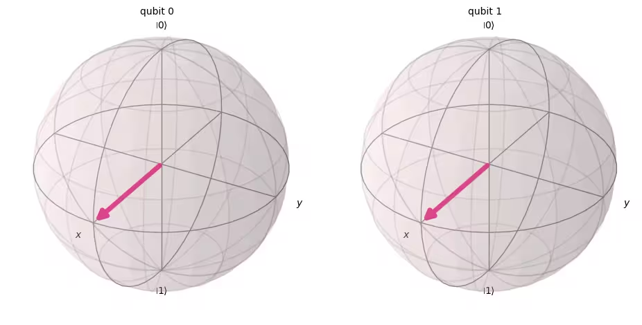
次のコードで 2 量子ビットの量子回路を作成できます。各量子ビットに H ゲートを適用します。

# Create the two qubits quantum circuit
qc = QuantumCircuit(2)

# Apply an H gate to qubit 0
qc.h(0)

# Apply an H gate to qubit 1
qc.h(1)

# Draw the circuit
qc.draw(output="mpl")

# See the statevector
out_vector = Statevector(qc)
print(out_vector)

Statevector([0.5+0.j, 0.5+0.j, 0.5+0.j, 0.5+0.j],
            dims=(2, 2))

注意：Qiskit のビット順序

Qiskit は量子ビットとビットの順序にリトルエンディアン表記を使用しており、量子ビット 0 はビット列の最も右側のビットとなります。例：$|01\rangle$ は q0 が $|1\rangle$、q1 が $|0\rangle$ であることを意味します。量子コンピューティングの一部の文献ではビッグエンディアン表記（量子ビット 0 が最も左のビット）が使用されており、量子力学の文献でも同様の場合が多いため、注意が必要です。

また、量子回路を表現する際、$|q_0\rangle$ は常に回路の一番上に配置されます。 これを踏まえると、上記の回路の量子状態は単一量子ビットの量子状態のテンソル積として記述できます。

$|q1\rangle \otimes|q0\rangle = (a|0\rangle+b|1\rangle) \otimes (c|0\rangle+d|1\rangle)$

$= ac|0\rangle|0\rangle+ad|0\rangle|1\rangle+bc|1\rangle|0\rangle+bd|1\rangle|1\rangle$

$= ac|00\rangle+ad|01\rangle+bc|10\rangle+bd|11\rangle$

( $|ac|^2+ |ad|^2+ |bc|^2+ |bd|^2=1$ )

Qiskit の初期状態は $|0\rangle|0\rangle=|00\rangle$ であり、各量子ビットに $H$ を適用すると等しい重ね合わせ状態に変化します。

$H|0\rangle \otimes H|0\rangle=\frac{1}{\sqrt{2}}(|0\rangle+|1\rangle) \otimes \frac{1}{\sqrt{2}}(|0\rangle+|1\rangle) = \frac{1}{2}(|00\rangle+|01\rangle+|10\rangle+|11\rangle)$

$$=\frac{1}{2}\left( \begin{pmatrix} 1 \\ 1 \end{pmatrix} \otimes \begin{pmatrix} 1 \\ 1 \end{pmatrix}\right) = \frac{1}{2}\begin{pmatrix} 1 \\ 1 \\ 1 \\ 1 \end{pmatrix}=\frac{1}{2}\left(\begin{pmatrix} 1 \\ 0 \\ 0 \\ 0 \end{pmatrix}+\begin{pmatrix} 0 \\ 1 \\ 0 \\ 0 \end{pmatrix}+\begin{pmatrix} 0 \\ 0 \\ 1 \\ 0 \end{pmatrix}+\begin{pmatrix} 0 \\ 0 \\ 0 \\ 1 \end{pmatrix}\right)$$

測定の規則は単一量子ビットの場合と同じで、$|00\rangle$ が測定される確率は $|ac|^2$ です。

# Draw a Bloch sphere
plot_bloch_multivector(out_vector)

次に、この回路を測定してみましょう。

# Create a new circuit with two qubits (first argument) and two classical bits (second argument)
qc = QuantumCircuit(2, 2)

# Apply the gates
qc.h(0)
qc.h(1)

# Add the measurement gates
qc.measure(0, 0)  # Measure qubit 0 and save the result in bit 0
qc.measure(1, 1)  # Measure qubit 1 and save the result in bit 1

# Draw the circuit
qc.draw(output="mpl")

次に、Aer シミュレータを再び使用して、すべての可能な出力状態の相対確率がほぼ等しいことを実験的に確認します。

# Run the circuit on a simulator to get the results
# Define backend
backend = AerSimulator()

# Transpile to backend
pm = generate_preset_pass_manager(backend=backend, optimization_level=1)
isa_qc = pm.run(qc)

# Run the job
sampler = Sampler(mode=backend)
job = sampler.run([isa_qc])
result = job.result()

# Print the results
counts = result[0].data.c.get_counts()
print(counts)

# Plot the counts in a histogram
plot_histogram(counts)

{'10': 262, '01': 246, '00': 265, '11': 251}

期待通り、$|00\rangle$、$|01\rangle$、$|10\rangle$、$|11\rangle$ の各状態がほぼ 25% ずつ測定されました。

4.2 複数量子ビットの量子ゲート

CNOTゲート

CNOTゲート（「制御NOTゲート」またはCXゲート）は2量子ビットゲートです。つまり、その動作は制御量子ビットとターゲット量子ビットの2つの量子ビットに同時に作用します。CNOTゲートは、制御量子ビットが $|1\rangle$ のときのみ、ターゲット量子ビットを反転させます。

入力 (ターゲット, 制御)	出力 (ターゲット, 制御)
00	00
01	11
10	10
11	01

まず、q0とq1の両方が $|0\rangle$ であるときに、この2量子ビットゲートの動作をシミュレートし、出力の状態ベクトルを求めてみましょう。使用するQiskitの構文は qc.cx(制御量子ビット, ターゲット量子ビット) です。

# Create a circuit with two quantum registers and two classical registers
qc = QuantumCircuit(2, 2)

# Apply the CNOT (cx) gate to a |00> state.
qc.cx(0, 1)  # Here the control is set to q0 and the target is set to q1.

# Draw the circuit
qc.draw(output="mpl")

# See the statevector
out_vector = Statevector(qc)
print(out_vector)

Statevector([1.+0.j, 0.+0.j, 0.+0.j, 0.+0.j],
            dims=(2, 2))

予想通り、$|00\rangle$ にCNOTゲートを適用しても状態は変化しませんでした。これは制御量子ビットが $|0\rangle$ の状態にあるためです。 次に、CNOT演算に戻ります。今度は $|01\rangle$ にCNOTゲートを適用して、何が起きるかを見てみましょう。

qc = QuantumCircuit(2, 2)

# q0=1, q1=0
qc.x(0)  # Apply a X gate to initialize q0 to 1
qc.cx(0, 1)  # Set the control bit to q0 and the target bit to q1.

# Draw the circuit
qc.draw(output="mpl")

# See the statevector
out_vector = Statevector(qc)
print(out_vector)

Statevector([0.+0.j, 0.+0.j, 0.+0.j, 1.+0.j],
            dims=(2, 2))

CNOTゲートを適用することで、$|01\rangle$ の状態が $|11\rangle$ に変化しました。

シミュレーターで回路を実行し、これらの結果を確認してみましょう。

# Add measurements
qc.measure(0, 0)
qc.measure(1, 1)

# Draw the circuit
qc.draw(output="mpl")

# Run the circuit on a simulator to get the results
# Define backend
backend = AerSimulator()

# Transpile to backend
pm = generate_preset_pass_manager(backend=backend, optimization_level=1)
isa_qc = pm.run(qc)

# Run the job
sampler = Sampler(backend)
job = sampler.run([isa_qc])
result = job.result()

# Print the results
counts = result[0].data.c.get_counts()
print(counts)

# Plot the counts in a histogram
plot_histogram(counts)

{'11': 1024}

結果を見ると、$|11\rangle$ が100%の確率で測定されていることが確認できます。

4.3 量子もつれと実機での実行

まず、量子計算において特に重要なもつれ状態を紹介し、その後「もつれ」という用語を定義します。

$$\frac{1}{\sqrt{2}}|00\rangle + \frac{1}{\sqrt{2}}|11\rangle$$

この状態はベル状態と呼ばれます。

もつれ状態とは、量子状態 $|\psi_A\rangle$ と $|\psi_B\rangle$ からなる状態 $|\psi_{AB}\rangle$ であり、個々の量子状態のテンソル積では表現できないものです。

以下の $|\psi_{AB}\rangle$ が2つの状態 $|\psi\rangle_A$ と $|\psi\rangle_B$ を持つとします。

$$|\psi_{AB}\rangle = \frac{1}{\sqrt{2}}(|00\rangle +|11\rangle) = \frac{1}{\sqrt{2}}(|0\rangle_A|0\rangle_B +|1\rangle_A|1\rangle_B)$$ $$|\psi\rangle_A = a_0|0\rangle+a_1|1\rangle$$ $$|\psi\rangle_B = b_0|0\rangle+b_1|1\rangle$$

これら2つの状態のテンソル積は次のようになります。

$$|\psi\rangle _A\otimes |\psi\rangle _B = a_0 b_0|00\rangle+a_0 b_1|01\rangle+a_1 b_0|10\rangle+a_1 b_1|11\rangle$$

しかし、この2つの方程式を同時に満たす係数 $a_0, a_1, b_0,$ および $b_1$ は存在しません。したがって、$|\psi_{AB}\rangle$ は個々の量子状態 $|\psi\rangle_A$ と $|\psi\rangle_B$ のテンソル積では表現できません。これは、$|\psi_{AB}\rangle = \frac{1}{\sqrt{2}}(|00\rangle +|11\rangle)$ がもつれ状態であることを意味しています。

ベル状態を生成し、実際の量子コンピューターで実行してみましょう。ここでは、Qiskitパターンと呼ばれる量子プログラムを書くための4つのステップに従います。

1. 問題を量子回路と演算子にマッピングする
2. ターゲットハードウェア向けに最適化する
3. ターゲットハードウェアで実行する
4. 結果を後処理する

ステップ1：問題を量子回路と演算子にマッピングする

量子プログラムにおいて、量子回路は量子命令を表現するためのネイティブなフォーマットです。回路を作成するときは、通常、新しい QuantumCircuit オブジェクトを作成し、そこに命令を順番に追加していきます。

次のコードセルは、上で紹介した特定の2量子ビットのもつれ状態であるベル状態を生成する回路を作成します。

qc = QuantumCircuit(2, 2)

qc.h(0)
qc.cx(0, 1)

qc.measure(0, 0)
qc.measure(1, 1)

qc.draw("mpl")

ステップ2：ターゲットハードウェア向けに最適化する

Qiskitは抽象的な回路を、ターゲットハードウェアの制約を考慮したQISA（量子命令セットアーキテクチャ）回路に変換し、回路のパフォーマンスを最適化します。最適化の前に、ターゲットハードウェアを指定します。 qiskit-ibm-runtime がインストールされていない場合は、最初にインストールする必要があります。Qiskit Runtimeの詳細については、APIリファレンスをご確認ください。

# Install
# !pip install qiskit-ibm-runtime

ターゲットハードウェアを指定します。

from qiskit_ibm_runtime import QiskitRuntimeService

service = QiskitRuntimeService()
service.backends()

# You can specify the device
# backend = service.backend('ibm_kingston')

# You can also identify the least busy device
backend = service.least_busy(operational=True)
print("The least busy device is ", backend)

回路のトランスパイルは、また別の複雑なプロセスです。簡単に言うと、回路を「ネイティブゲート」（特定の量子コンピューターが実行できるゲート）を使って論理的に等価な回路に書き換え、回路内の量子ビットをターゲット量子コンピューター上の最適な実量子ビットにマッピングします。トランスパイルの詳細については、こちらのドキュメントをご覧ください。

# Transpile the circuit into basis gates executable on the hardware
pm = generate_preset_pass_manager(backend=backend, optimization_level=1)
target_circuit = pm.run(qc)

target_circuit.draw("mpl", idle_wires=False)

トランスパイルによって回路が新しいゲートを使って書き換えられていることが確認できます。詳細については、ECRGate のドキュメントをご参照ください。

ステップ3：ターゲット回路を実行する

では、実機でターゲット回路を実行します。

sampler = Sampler(backend)
job_real = sampler.run([target_circuit])

job_id = job_real.job_id()
print("job id:", job_id)

量子コンピューターは貴重なリソースで需要が非常に高いため、実機での実行にはキューでの待機が必要になる場合があります。job_id は、後でジョブの実行状態と結果を確認するために使用します。

# Check the job status (replace the job id below with your own)
job_real.status(job_id)

IBM Quantumのダッシュボードからジョブの状態を確認することもできます：https://quantum.cloud.ibm.com/workloads

# If the Notebook session got disconnected you can also check your job status by running the following code
from qiskit_ibm_runtime import QiskitRuntimeService

service = QiskitRuntimeService()
job_real = service.job(job_id)  # Input your job-id between the quotations
job_real.status()

# Execute after job has successfully run
result_real = job_real.result()
print(result_real[0].data.c.get_counts())

ステップ4：結果を後処理する

最後に、結果を値やグラフなど期待される形式の出力に変換するために後処理を行います。

plot_histogram(result_real[0].data.c.get_counts())

ご覧のように、$|00\rangle$ と $|11\rangle$ が最も頻繁に観測されています。期待されるデータ以外にもいくつかの結果が含まれていますが、これはノイズと量子ビットのデコヒーレンスによるものです。量子コンピューターにおけるエラーとノイズについては、このコースの後続レッスンでさらに詳しく学びます。

4.4 GHZ状態

もつれの概念は、2量子ビットを超えるシステムにも拡張できます。GHZ状態（Greenberger-Horne-Zeilinger状態）は、3つ以上の量子ビットの最大もつれ状態です。3量子ビットのGHZ状態は次のように定義されます。

$$\frac{1}{\sqrt 2}(|000\rangle + |111\rangle)$$

これは以下の量子回路で生成できます。

qc = QuantumCircuit(3, 3)

qc.h(0)
qc.cx(0, 1)
qc.cx(1, 2)

qc.measure(0, 0)
qc.measure(1, 1)
qc.measure(2, 2)

qc.draw("mpl")

量子回路の「深さ（デプス）」は、量子回路を説明するための有用でよく使われる指標です。量子回路を左から右へとたどり、複数量子ビットのゲートで接続されているときのみ量子ビットを切り替えます。そのパス上のゲートの数を数えます。回路を通るあらゆるパスにおけるゲート数の最大値がデプスです。現代のノイズのある量子コンピューターでは、デプスの浅い回路ほどエラーが少なく、良好な結果が得られやすいです。非常に深い回路はそうではありません。

QuantumCircuit.depth() を使って量子回路のデプスを確認できます。上記の回路のデプスは4です。最上位の量子ビットは測定を含め3つのゲートしか持ちませんが、最上位の量子ビットから量子ビット1または量子ビット2へのパスにはさらにCNOTゲートが含まれます。

qc.depth()

4

演習2

8量子ビットシステムのGHZ状態は次のとおりです。

$$\frac{1}{\sqrt 2}(|00000000\rangle + |11111111\rangle)$$

できるだけ浅い回路でこの状態を準備するコードを書いてください。測定ゲートを含む最も浅い量子回路のデプスは5です。

解答:

# Step 1
qc = QuantumCircuit(8, 8)

##your code goes here##
qc.h(0)
qc.cx(0, 4)
qc.cx(4, 6)
qc.cx(6, 7)

qc.cx(4, 5)

qc.cx(0, 2)
qc.cx(2, 3)

qc.cx(0, 1)
qc.barrier()  # for visual separation

# measure
for i in range(8):
    qc.measure(i, i)

qc.draw("mpl")
# print(qc.depth())

print(qc.depth())

5

from qiskit.visualization import plot_histogram
# Step 2
# For this exercise, the circuit and operators are simple, so no optimizations are needed.

# Step 3
# Run the circuit on a simulator to get the results
backend = AerSimulator()

pm = generate_preset_pass_manager(backend=backend, optimization_level=1)
isa_qc = pm.run(qc)

sampler = Sampler(mode=backend)
job = sampler.run([isa_qc], shots=1024)
result = job.result()

counts = result[0].data.c.get_counts()
print(counts)

# Step 4
# Plot the counts in a histogram

plot_histogram(counts)

{'11111111': 535, '00000000': 489}

5. まとめ

量子ビットとゲートを用いた回路モデルによる量子計算を学び、重ね合わせ、測定、もつれについて復習しました。また、実際の量子デバイスで量子回路を実行する方法も学びました。

GHZ回路を作成する最後の演習では、回路のデプスを削減しようとしました。これは、ノイズのある量子コンピューターでユーティリティスケールの解を得るための重要な要素です。このコースの後続レッスンでは、ノイズとエラー軽減手法について詳しく学びます。このレッスンでは入門として理想的なデバイスにおける回路デプスの削減を考えましたが、実際には量子ビット接続性などの実デバイスの制約も考慮する必要があります。これについては、このコースの後続レッスンでさらに詳しく学びます。

# See the version of Qiskit
import qiskit

qiskit.__version__

'2.0.2'