ユーティリティスケールQAOA

Olivia LanesによるユーティリティスケールQAOAに関する動画をご覧ください。またはYouTubeで別ウィンドウで開くこともできます。

レッスンの概要

このコースのここまでの内容で、量子コンピューターでユーティリティスケールの問題を解くために必要なフレームワークとツールの確固たる基礎をお伝えできたと思います。いよいよ、これらのツールを実際に動かしてみましょう。

このレッスンでは、グラフをどのように最適に2つに分割するかを問うグラフ理論の有名な問題、Max-Cut問題のユーティリティスケールの例に取り組みます。まずは5ノードのシンプルなグラフから始め、量子コンピューターがこの問題の解決にどのように役立つかの直感を養い、その後ユーティリティスケール版の問題に応用します。

このレッスンは、この問題へのアプローチの大まかな概要となります。コードのウォークスルーではありません。ただし、このレッスンに対応するチュートリアルがあり、量子コンピューター上でMax-Cut問題を実際に解けるコードが含まれています。

問題

まず確認しておくと、すべての計算問題が量子コンピューティングに適しているわけではありません。「簡単な問題」は、古典コンピューターがすでに十分に解けるため、この技術から恩恵を受けることはありません。

私たちが最も期待を寄せて探求している3つのユースケースは次の通りです。

1. 自然のシミュレーション
2. 複雑な構造を持つデータの処理
3. 最適化

今日は3番目のユースケースである最適化に焦点を当てます。最適化問題では、一般的にある関数の最大値または最小値を探します。古典的な手法でこれらの極値を見つける難しさは、問題のサイズが大きくなるにつれて指数関数的に増大します。

今日取り上げる最適化問題はMax-Cutと呼ばれるもので、量子近似最適化アルゴリズム（QAOA）を使って解きます。

Max-Cutとは？

グラフとは、頂点（またはノード）の集まりであり、その一部がエッジで接続されています。この問題では、エッジを「切断」することでグラフのノードを2つのサブセットに分割するよう求められます。このようにカットされるエッジの数を最大化する分割を見つけることが目的です。これが「Max-Cut」という名前の由来です。

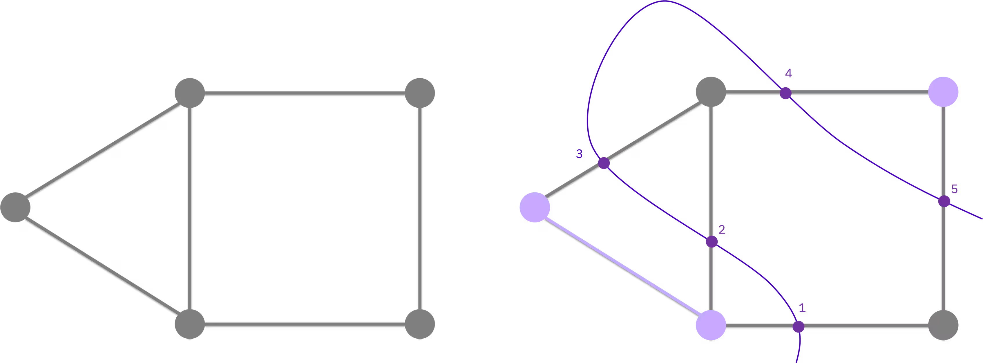
たとえば、上の図は5ノードのグラフと、右側にMax-Cut解を示しています。5本のエッジを切断しており、このグラフで達成できる最良の結果です。

5ノードのグラフは非常に小さいため、頭の中や紙に何度かカットを試みることでMax-Cutを求めることはそれほど難しくありません。しかし、頂点の数が増えるにつれて問題はどんどん難しくなります。考えうるカットの数がノード数に対して指数関数的に増大するためです。ある時点からは、既知の古典アルゴリズムではスーパーコンピューターでさえ解くのが困難になります。

より大きく複雑なグラフに対してMax-Cut問題を解く方法が求められています。この問題は金融における不正検出、グラフクラスタリング、ネットワーク設計、ソーシャルメディア分析など多くの実用的な応用があります。Max-Cutは、より大きな問題の特定のアプローチにおけるサブ問題としてよく登場します。そのため、私たちが単純に思う以上に一般的な問題なのです。

解法

これから、量子コンピューター上でMax-Cut問題を解くためのアプローチを5ノードのシンプルなグラフで説明していきます。Pythonノートブックのチュートリアルを参照しながら進めることができます。そのシンプルな例の後、チュートリアルではユーティリティスケールの例も扱います。

最初のステップは、ノード数とノード同士を接続するエッジを定義してグラフを作成することです。チュートリアルで示されているように、rustworkxというパッケージをインポートすることで実現できます。結果として、次のようなグラフが得られます。

Qiskitパターンズフレームワークを使って、このグラフのMax-Cut解を量子コンピューターで求めます。

マッピング

問題を量子コンピューターにマッピングする必要があります。そのためにまず、グラフのカット数の最大化は数学的に次のように表せることに注目します。

$$\max\limits_{x\in\{0,1\}^n} \sum\limits_{(i,j)} {x_i + x_j - 2x_ix_j}$$

ここで$i$と$j$はグラフのノードを表し、$x_i$と$x_j$は各ノードがどちらの分割側にあるかによって0または1の値をとります（一方のグループを「0」、もう一方を「1」とラベル付けします）。$x_i$と$x_j$が同じ側にある場合、和の中の式はゼロになります。反対側にある場合（つまりカットがある場合）、式は1になります。よって、カット数を最大化することが和を最大化することになります。

各値に−1を掛けることで最小化問題に変換することもできます。

$$\min\limits_{x\in\{0,1\}^n} \sum\limits_{(i,j)} {2x_ix_j - x_i - x_j}$$

これでマッピングの準備ができました。グラフから量子回路にどう変換するかを考えると少し戸惑うかもしれませんが、一歩ずつ進めていきましょう。

Max-CutをQAOAを使って解こうとしていることを思い出してください。QAOAの方法論では、最終的にハイブリッドアルゴリズムのコスト関数を表す演算子（つまりハミルトニアン）と、問題の候補解を表すパラメータ化回路（アンザッツ）が必要です。

QUBO

これらの候補解からサンプリングし、コスト関数で評価することができます。そのために、組み合わせ最適化問題を符号化するのに役立つ二値二次計画法（QUBO）表記を含む一連の数学的変換を活用します。QUBOでは次を求めます。

$$\min\limits_{x\in\{0,1\}^n} x^TQx$$

ここで$Q$は実数の$n\times n$行列であり、$n$はグラフのノード数（ここでは5）に対応します。

QAOAを適用するには、問題をハミルトニアン、つまりシステムの全エネルギーを表す関数または行列として定式化する必要があります。具体的には、基底状態が関数の最小値に対応するコスト関数ハミルトニアンを作成します。よって最適化問題を解くために、量子コンピューター上で$H$の基底状態を準備しようとします。この状態からサンプリングすることで、$\min 𝑓(𝑥)$の解を高い確率で得られます。

コスト関数ハミルトニアンへのマッピング

幸いなことに、QUBO問題は物理学で最も有名で普遍的なハミルトニアンの一つであるイジングハミルトニアンと非常に近く、実際に計算量的に等価です。

QUBO問題をイジングハミルトニアンとして書くには、単純な変数置換を行うだけです。

$$x_i = \frac{1-z_i}{2}.$$

ここではすべてのステップを説明しませんが、添付のノートブックで詳しく解説されています。最終的に、QUBO式の最小化とこの式の最小化は等価です。

$$\min_{x\in\{0,1\}^n} x^TQx\Longleftrightarrow \min_{z\in\{-1,1\}^n}z^TQz + b^Tz$$

少し書き直すと、コスト関数ハミルトニアンが得られます。ここで式の最小値が基底状態を表し、ZはパウリZ演算子、$b$は実スカラー係数です。

$$H_C=\sum_{ij}Q_{ij}Z_iZ_j + \sum_i b_i Z_i$$

ハミルトニアンが得られたら、量子回路の2量子ビットゲートに変換しやすい2局所パウリZZ演算子の形に書き直す必要があります。グラフの6本のエッジに対応する6つのオブジェクト（パウリ文字列）が得られます。各文字列の5つの要素はそれぞれのノードへの操作を表します。そのエッジに接続されていないノードには恒等演算子、接続されているノードにはパウリZ演算子が対応します。Qiskitでは、量子ビットを表すビット列は逆順にインデックスされます。たとえば、ノード0と1の間のエッジはIIIZZとして符号化され、ノード2と4の間のエッジはZIZIIとして符号化されます。

量子回路の構築

パウリ演算子で書かれたハミルトニアンが得られたので、量子コンピューターを使って良い解をサンプリングできる量子回路を構築する準備ができました。

QAOAアルゴリズムは断熱定理からヒントを得ています。断熱定理とは、時間依存ハミルトニアンの基底状態から始まり、ハミルトニアンがゆっくりと変化し、十分な時間が与えられれば、最終状態は最終ハミルトニアンの基底状態になるというものです。QAOAは量子断熱アルゴリズムの離散的なトロッター化バージョンと考えることができ、各トロッターステップがQAOAアルゴリズムの1つのレイヤーに対応します。つまり一方の状態から他方へと連続的に発展するのではなく、各レイヤーでコスト関数ハミルトニアンと後述する「ミキサー」ハミルトニアンを交互に切り替えます。

QAOAの利点は量子断熱アルゴリズムより高速であることですが、最適解ではなく近似解を返します。レイヤー数が無限大に近づく極限では、QAOAはQAAの場合に収束しますが、これは計算コストが非常に高くなります。

量子回路を作成するために、$\gamma$と$\beta$でパラメータ化された交互演算子を適用し、時間発展の離散化を表現します。

QAOA回路の主な3つの部分は次の通りです。

1. グレーで示した初期試行状態。ミキサーの基底状態であり、すべての量子ビットにアダマールゲートを適用することで作成されます。
2. 濃い紫で示した、前述したコスト関数の発展。
3. 薄い紫で示した、ミキサーハミルトニアンによる発展（まだ説明していません）。

開始ハミルトニアンをミキサーと呼ぶのは、その基底状態が関心のあるすべての可能なビット列の重ね合わせであり、最初に全候補解の混合を強制するためです。

ミキサーハミルトニアンは、グラフの各ノードへのパウリX演算の単純な和です。Qiskitでは必要に応じて異なるカスタムミキサー演算子を使用できますが、ここでは標準的なものを使います。このようにQiskitを使うことで多くの作業が省かれ、ミキサーハミルトニアンと開始状態の構築が容易になります。私たちがする必要があった唯一の作業は、コスト関数を求めることだけです。

これらの演算子の各反復をレイヤーと呼びます。これらのレイヤーは前述のように、システムの時間発展の離散化と見なすことができます。交互パターンはトロッター分解から来ており、非可換行列の指数関数を近似します。一般的に、レイヤー（ステップ）が多ければ多いほど、QAAのような連続時間発展に近づき、理論上は結果がより正確になります。ただしこの例では、まず1レイヤーでサンプリングから始めます。コスト関数ハミルトニアンとミキサーの両方がパラメータ化されているため、$\gamma$と$\beta$の最適値をまだ決める必要があります。

最適化

今作成した回路はシンプルで直感的な理解を構築するのに役立ちますが、量子チップはQAOAゲートが何であるかを理解していません。これをハードウェア上で直接実行できる1量子ビットおよび2量子ビットの「ネイティブ」ゲートの列に変換する必要があります。ネイティブゲートとは、量子ビット上で直接実行できるゲートのことです。そのような回路はバックエンドの命令セットアーキテクチャ（ISA）で書かれていると言われます。

Qiskitライブラリは、幅広い回路変換に対応するトランスパイルパスを提供しています。回路が私たちの目的に最適化されていることを確認する必要があります。

前のレッスンで学んだように、トランスパイルプロセスには次のいくつかのステップが含まれます。

• 回路内の量子ビット（つまり決定変数）をデバイス上の物理量子ビットに初期マッピングする。
• 量子回路内の命令をバックエンドが理解できるハードウェアネイティブ命令に展開する。
• 相互作用する回路内の量子ビットを、互いに隣接する物理量子ビットへルーティングする。

詳細はいつものようにドキュメントで確認できます。

ただし、トランスパイルの前に、実行するバックエンドを選択する必要があります。トランスパイラーはプロセッサーによって最適化方法が異なるためです。これが自動トランスパイラーを使用することが重要なもう一つの理由です。手作業で時間をかけて回路を最適化した後に、異なるプロセッサーで実行したいと気づいた場合、最初からやり直しになってしまいます。

選択したバックエンドをトランスパイラー関数に渡し、最適化レベルを指定します。チュートリアルでは最高レベルで最も徹底的なレベル3を選択します。

これで、ハードウェアで実行できる状態のトランスパイル済み回路が完成しました！

実行

ここまでで、パラメータのgammaとbetaをそのままにして回路をトランスパイルしましたが、これらのパラメータを指定しなければ実際には回路を実行できません。QAOAのワークフローでは、最適なQAOAパラメータは反復最適化ループで求められます。一連の回路評価を実行し、古典オプティマイザーを使って最適な𝛽と𝛾のパラメータを見つけます。ただし、どこかから始める必要があるため、$\gamma=\pi/2$、$\beta=\pi$を初期推測値として使います。

実行モード

さあ、回路を実行する準備がほぼ整いました。しかしその前に、ジョブを送信するいくつかの方法（実行モードと呼ばれます）があることを確認しておきましょう。

• ジョブモード：コンテキストマネージャーを使わずに、エスティメーターまたはサンプラーへの単一のプリミティブリクエストが行われます。回路と入力はプリミティブユニファイドブロック（PUB）としてパッケージ化され、量子コンピューターの実行タスクとして送信されます。

• バッチモード：独立したジョブの束から構成される実験を効率的に実行するためのマルチジョブマネージャーです。バッチモードを使用して、複数のプリミティブジョブを同時に送信できます。

• セッションモード：マルチジョブワークロードを実行するための専用ウィンドウです。ユーザーが変分アルゴリズムをより予測可能な方法で試せ、スタックの並列性を活用して複数の実験を同時に実行することもできます。専用アクセスが必要な反復的なワークロードや実験にはセッションを使用してください。例については「セッションでのジョブ実行」をご覧ください。

QAOAの実験では、最適値を見つけるために異なるパラメータ値で回路を何度もサンプリングする必要があるため、アクセスできるのであればセッションを選択するのが良いでしょう。

最適化問題に戻りましょう。gammaとbetaの最初のおおまかな推測よりも良い値を見つける必要があります。コスト関数とこれらの初期推測値をscipyオプティマイザーCOBYLAに入力することで実現します。

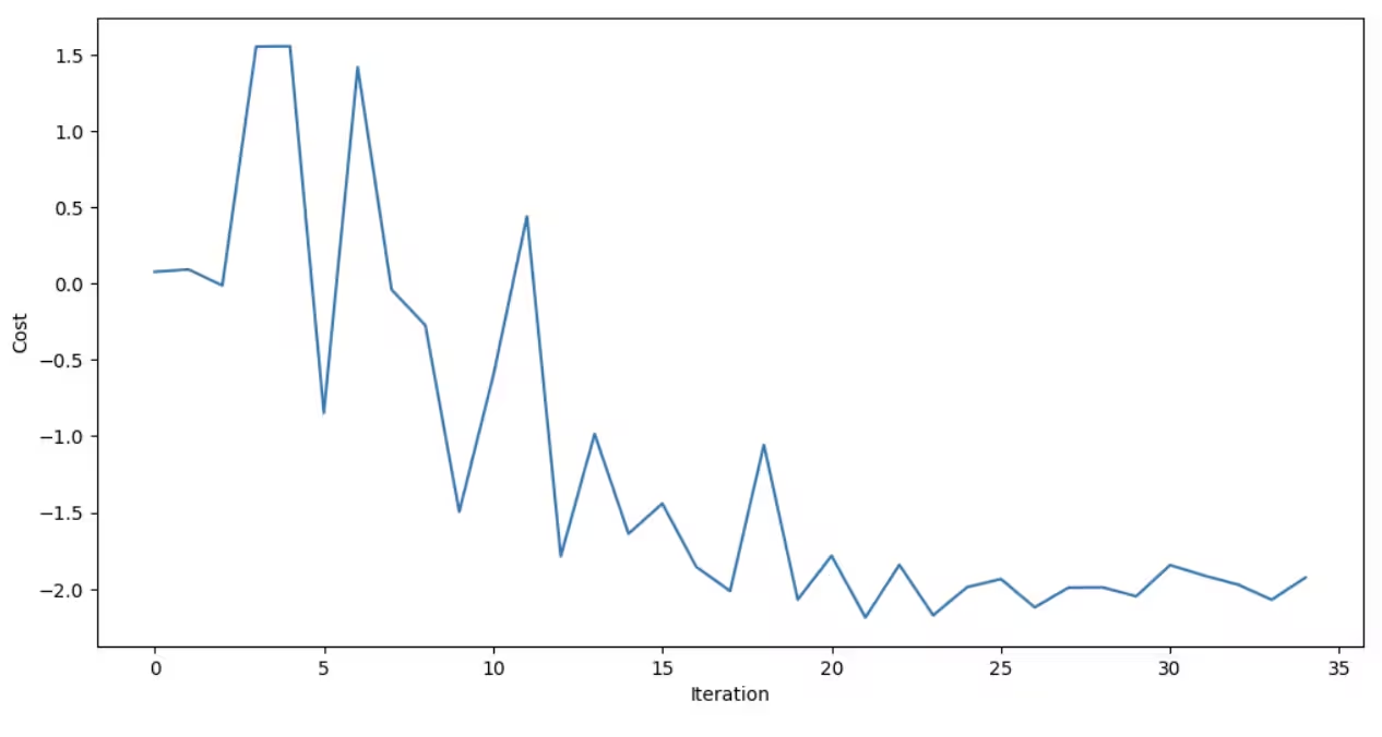
ここでは、反復回数に対するコスト関数の値を確認できます。最初は多少不安定で上下しますが、やがて低い値に落ち着きます。コスト関数の評価が最も低くなる値をscipyが見つけた値として使用します。

パラメータの最適化によりコスト関数を下げることができたので、gammaとbetaの新しい値を使って回路を実行します。ここで使用している具体的な値を示しましたが、同じチュートリアルノートブックを試したり再実行したりする場合、これらの値は若干変わる可能性があります。最適化した回路をこれらの値で実行し、Max-Cut問題の候補解を見つけます。

後処理段階では、データを分析してこれらの結果を表示し、量子アルゴリズムが正しい解を見つけられたかを確認します。

後処理

最終解を確認するために、データのヒストグラムをプロットしましょう。

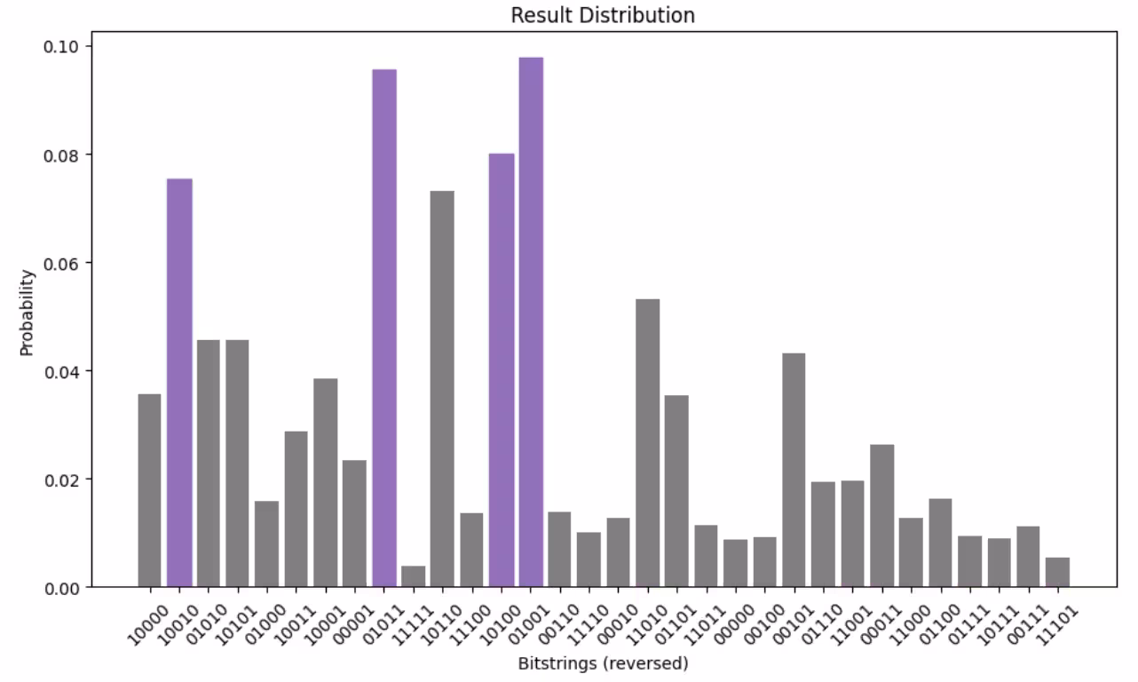
ビット列は、各ノードがカットによってどのように2つのグループ（「0」と「1」とラベル付けされた）に分割されたかを表しています。カットされるエッジの数が最大となる解は4つあるはずです。これらの4つは紫色で示されています。すぐにわかるように、4つの解は他のどの解よりも確率が高くなっています。最も高く、したがって最も確率の高いビット列解は0,1,0,1,1です（プロットのビット列では量子ビットの順序が逆になっていることを覚えておいてください！）。

このプロットから、最も確率の高いビット列を取り出し、5本のエッジを切断するパーティション分割されたグラフとして表現できます。

これは確かにMax-Cut解です。しかし、これが唯一の解ではありません。このグラフの対称性のために、複数の正しい解が存在します。ノード0と3がカットの内側にある代わりに、ノード2と4が含まれる場合もあります。カットを回転させてこれらの新しい点を含めるだけです。カットされるエッジの数は変わらず5本です。実際には4つのMax-Cut解があります。指摘した2つの解のそれぞれに「反対」のパターンがあり、紫のノードがグレーに、グレーのノードが紫になります。つまりカットは同じですが、各ノードは実質的に分割の反対側に入れ替わります。

再びヒストグラムと上位4つの最も確率の高い解を見てみましょう。理想的には、それぞれが4つの真のMax-Cut解であるはずです。問題は、アルゴリズムが実際には4番目の最後の解を上位4つの最も確率の高い答えの一つとして識別しなかったことです。それは5番目に確率が高い解でした。アルゴリズムが識別した4番目の解は誤りです。描いてみると、その解はわずか4つのカットしかないことがわかります。

ただし、これは近似アルゴリズムであることを覚えておいてください。絶対に正しいわけではなく、100%正確というわけでもありません。解の妥当性を確認するためには、自分自身の知識と理解を活用する必要があります。

このエラーはいくつかの原因で生じる可能性があります。

1. アルゴリズム自体の近似的な性質と、使用したレイヤー数が少ないこと。
2. 有限サンプリング誤差。実験のショット数を増やすことで軽減できます。
3. 読み出しエラー。4番目の真の解はわずか1ビットだけ異なるためです。

このような誤差分析こそが、量子コンピューティングの実践者になるために必要なことです。ハードウェアの性能を理解し、それが特定のタイプのエラーにどのように寄与するか、そしてそれらをどのように修正するかを理解する必要があります。

ただし、32通りの可能なビット列があり、4つの真の解が上位5つの候補の中に含まれていたことを忘れないでください。しかも、これはわずか2レイヤーを使って見つけたものです。一般的に、常に最良のMax-Cutを見つける確率を高めたい場合は、レイヤーの深さを増やすことができます。いくつかの細かい点がありますが、それは後のレッスンで扱います。

ユーティリティスケールで

小さなMax-Cut問題を量子コンピューターで解くプロセスを体験したところで、今度はスケールアップに挑戦してみましょう。リンクされたチュートリアルに従って、125ノードのグラフでいくつのカットが得られるかを確認してください。