Gate CuttingによるCircuit幅の削減

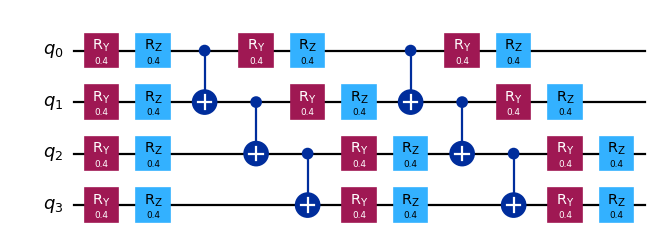
このノートブックでは、circuit cuttingを使用してCircuit内のQubit数を削減しながら、Qiskit patternの手順を実践していきます。Gateを切断することで、2-Qubit実験のみを使用して4-QubitのCircuitの期待値を再構成できるようにします。

実施する手順は以下の通りです：

• ステップ1：問題を量子Circuit・演算子にマッピングする：
  • ハミルトニアンを量子Circuitにマッピングします。
• ステップ2：ターゲットハードウェア向けに最適化する [cutting addonを使用]：
  • CircuitとObservableを切断します。
  • ハードウェア向けにサブ実験をトランスパイルします。
• ステップ3：ターゲットハードウェアで実行する：
  • Sampler primitiveを使用して、ステップ2で得られたサブ実験を実行します。
• ステップ4：結果を後処理する [cutting addonを使用]：
  • ステップ3の結果を組み合わせて、対象のObservableの期待値を再構成します。

ステップ1：マッピング

切断するCircuitを作成する

# Added by doQumentation — required packages for this notebook
!pip install -q numpy qiskit qiskit-addon-cutting qiskit-aer qiskit-ibm-runtime

from qiskit.circuit.library import efficient_su2

qc = efficient_su2(4, entanglement="linear", reps=2)
qc.assign_parameters([0.4] * len(qc.parameters), inplace=True)

qc.draw("mpl", scale=0.8)

Observableを指定する

from qiskit.quantum_info import SparsePauliOp

observable = SparsePauliOp(["ZZII", "IZZI", "-IIZZ", "XIXI", "ZIZZ", "IXIX"])

ステップ2：最適化

指定されたQubitのパーティショニングに従ってCircuitとObservableを分割する

partition_labelsの各ラベルは、同じインデックスのcircuit Qubitに対応しています。共通のパーティション・ラベルを共有するQubitはグループ化され、複数のパーティションにまたがる非ローカルなGateは切断されます。

注意： partition_problemへのobservablesキーワード引数の型はPauliListです。Observableの項の係数と位相は、問題の分解とサブ実験の実行中は無視されます。これらは期待値の再構成時に再適用できます。

from qiskit_addon_cutting import partition_problem

partitioned_problem = partition_problem(
    circuit=qc, partition_labels="AABB", observables=observable.paulis
)
subcircuits = partitioned_problem.subcircuits
subobservables = partitioned_problem.subobservables
bases = partitioned_problem.bases

分解された問題を可視化する

subobservables

{'A': PauliList(['II', 'ZI', 'ZZ', 'XI', 'ZZ', 'IX']),
 'B': PauliList(['ZZ', 'IZ', 'II', 'XI', 'ZI', 'IX'])}

subcircuits["A"].draw("mpl", scale=0.8)

subcircuits["B"].draw("mpl", scale=0.8)

選択した切断箇所のサンプリング・オーバーヘッドを計算する

ここでは2つのCNOT Gateを切断するため、サンプリング・オーバーヘッドは $9^2$ になります。

circuit cuttingによって生じるサンプリング・オーバーヘッドの詳細については、解説資料を参照してください。

import numpy as np

print(f"Sampling overhead: {np.prod([basis.overhead for basis in bases])}")

Sampling overhead: 81.0

Backendで実行するサブ実験を生成する

generate_cutting_experimentsは、Qubitのパーティション・ラベルをそれぞれのsubcircuit/subobservablesにマッピングする辞書としてcircuits/observables引数を受け取ります。

フルサイズのCircuitの期待値をシミュレートするため、分解されたGateの結合準確率分布から多数のサブ実験が生成され、1つ以上のBackendで実行されます。分布からのサンプル数はnum_samplesで制御され、ユニークなサンプルごとに1つの結合係数が与えられます。係数の計算方法の詳細については、解説資料を参照してください。

from qiskit_addon_cutting import generate_cutting_experiments

subexperiments, coefficients = generate_cutting_experiments(
    circuits=subcircuits, observables=subobservables, num_samples=np.inf
)

Backendを選択する

ここではフェイク・Backendを使用しており、Qiskit Runtimeがローカル・モード（ローカル・シミュレーター上）で実行されます。

from qiskit_ibm_runtime.fake_provider import FakeManilaV2

backend = FakeManilaV2()

Backendのためにサブ実験を準備する

Qiskit Runtimeに送信する前に、Backendをターゲットとして回路をトランスパイルする必要があります。

from qiskit.transpiler import generate_preset_pass_manager

# Transpile the subexperiments to ISA circuits
pass_manager = generate_preset_pass_manager(optimization_level=1, backend=backend)
isa_subexperiments = {
    label: pass_manager.run(partition_subexpts)
    for label, partition_subexpts in subexperiments.items()
}

ステップ3：実行

Qiskit Runtime Sampler primitiveを使用してサブ実験を実行する

from qiskit_ibm_runtime import SamplerV2, Batch

# Submit each partition's subexperiments to the Qiskit Runtime Sampler
# primitive, in a single batch so that the jobs will run back-to-back.
with Batch(backend=backend) as batch:
    sampler = SamplerV2(mode=batch)
    jobs = {
        label: sampler.run(subsystem_subexpts, shots=2**12)
        for label, subsystem_subexpts in isa_subexperiments.items()
    }

/home/garrison/Qiskit/qiskit-ibm-runtime/qiskit_ibm_runtime/session.py:157: UserWarning: Session is not supported in local testing mode or when using a simulator.
  warnings.warn(

# Retrieve results
results = {label: job.result() for label, job in jobs.items()}

ステップ4：後処理

期待値を再構成する

各Observableの項の期待値を再構成し、それらを組み合わせて元のObservableの期待値を再構成します。

from qiskit_addon_cutting import reconstruct_expectation_values

# Get expectation values for each observable term
reconstructed_expval_terms = reconstruct_expectation_values(
    results,
    coefficients,
    subobservables,
)

# Reconstruct final expectation value
reconstructed_expval = np.dot(reconstructed_expval_terms, observable.coeffs)

再構成された期待値を元のCircuitとObservableの正確な期待値と比較する

from qiskit_aer.primitives import EstimatorV2

estimator = EstimatorV2()
exact_expval = estimator.run([(qc, observable)]).result()[0].data.evs
print(f"Reconstructed expectation value: {np.real(np.round(reconstructed_expval, 8))}")
print(f"Exact expectation value: {np.round(exact_expval, 8)}")
print(f"Error in estimation: {np.real(np.round(reconstructed_expval-exact_expval, 8))}")
print(
    f"Relative error in estimation: {np.real(np.round((reconstructed_expval-exact_expval) / exact_expval, 8))}"
)

Reconstructed expectation value: 0.6991539
Exact expectation value: 0.56254612
Error in estimation: 0.13660778
Relative error in estimation: 0.24283836