SQDを用いた化学ハミルトニアンのエネルギー推定の改善

このチュートリアルでは、Qiskit パターンを実装します。これは、ノイズの多い量子サンプルを後処理することで、化学ハミルトニアン（6-31G基底関数系における平衡状態の $N_2$ 分子）の基底状態の近似値を求める方法を示すものです。サンプルベースの量子対角化アプローチに従い、36 Qubit の量子 Circuit アンザッツ（この場合はLUCJ Circuit）から取得したサンプルを処理します。量子ノイズの影響を考慮するために、構成回復手法を使用します。

このパターンは4つのステップで説明できます。

ステップ1：量子問題へのマッピング
- 基底状態を推定するためのアンザッツを生成する
ステップ2：問題の最適化
- Backend 向けにアンザッツをトランスパイルする
ステップ3：実験の実行
- Sampler プリミティブを使用してアンザッツからサンプルを取得する
ステップ4：結果の後処理
- 自己無撞着構成回復ループ
  - 粒子数の事前知識と最新のイテレーションで計算された平均軌道占有率を使用して、ビット列サンプルの完全なセットを後処理する。
  - 回復されたビット列から確率的にサブサンプルのバッチを作成する。
  - 各サンプリングされた部分空間に対して分子ハミルトニアンを射影・対角化する。
  - 全バッチにわたって見つかった最小の基底状態エネルギーを保存し、平均軌道占有率を更新する。

この例では、相互作用電子ハミルトニアンは一般的な形式をとります：

\hat{H} = \sum_{ \substack{pr\\\sigma} } h_{pr} \, \hat{a}^\dagger_{p\sigma} \hat{a}_{r\sigma} + \sum_{ \substack{prqs\\\sigma\tau} } \frac{(pr|qs)}{2} \, \hat{a}^\dagger_{p\sigma} \hat{a}^\dagger_{q\tau} \hat{a}_{s\tau} \hat{a}_{r\sigma}

$\hat{a}^\dagger_{p\sigma}$ / $\hat{a}_{p\sigma}$ は、 $p$ 番目の基底関数要素とスピン $\sigma$ に関連するフェルミオン生成・消滅演算子です。 $h_{pr}$ および $(pr|qs)$ は1体および2体の電子積分です。

自己無撞着構成回復を用いたSQDワークフローを以下の図に示します。

SQD diagram

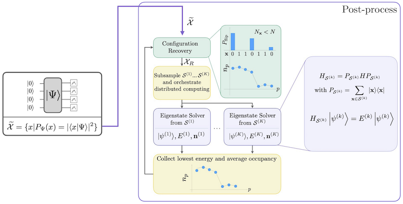
SQDは、ターゲット固有状態がスパースである場合に有効です。つまり、波動関数が基底状態の集合 $\mathcal{S} = \{|x\rangle \}$ に乗っており、その大きさが問題のサイズとともに指数関数的に増加しない場合です。このシナリオでは、 $\mathcal{S}$ で定義された部分空間に射影されたハミルトニアンの対角化：

H_\mathcal{S} = P_\mathcal{S} H P_\mathcal{S} \textrm{ with } P_\mathcal{S} = \sum_{x \in \mathcal{S}} |x \rangle \langle x |;

は、ターゲット固有状態の良い近似を与えます。量子デバイスの役割は、 $\mathcal{S}$ のメンバーのサンプルのみを生成することです。まず、量子 Circuit が量子デバイスで状態 $|\Psi\rangle$ を準備します。ジョルダン・ウィグナー符号化が使用されます。その結果、計算基底のメンバーはフォック状態（電子配置・行列式）を表します。Circuit は計算基底でサンプリングされ、ノイズを含む配置の集合 $\tilde{\mathcal{X}}$ が得られます。配置はビット列で表されます。集合 $\tilde{\mathcal{X}}$ は次に古典的な後処理ブロックに渡され、自己無撞着構成回復手法が使用されます。SQDフレームワークにおける量子デバイスの役割は、確率分布を生成することです。

ステップ1：問題を量子 Circuit にマッピングする

このチュートリアルでは、 $N_2$ 分子の基底状態エネルギーを近似します。まず、分子とその特性を指定します。次に、局所ユニタリー・クラスター・ジャストロウ（LUCJ）アンザッツ（量子 Circuit）を作成して、基底状態エネルギー推定のために量子コンピューターからサンプルを生成します。

まず、分子とその特性を指定します。

# Added by doQumentation — required packages for this notebook
!pip install -q ffsim matplotlib numpy pyscf qiskit qiskit-addon-sqd qiskit-ibm-runtime

import warnings

warnings.filterwarnings("ignore")

import pyscf
import pyscf.cc
import pyscf.mcscf

# Specify molecule properties
open_shell = False
spin_sq = 0

# Build N2 molecule
mol = pyscf.gto.Mole()
mol.build(
    atom=[["N", (0, 0, 0)], ["N", (1.0, 0, 0)]],
    basis="6-31g",
    symmetry="Dooh",
)

# Define active space
n_frozen = 2
active_space = range(n_frozen, mol.nao_nr())

# Get molecular integrals
scf = pyscf.scf.RHF(mol).run()
num_orbitals = len(active_space)
n_electrons = int(sum(scf.mo_occ[active_space]))
num_elec_a = (n_electrons + mol.spin) // 2
num_elec_b = (n_electrons - mol.spin) // 2
cas = pyscf.mcscf.CASCI(scf, num_orbitals, (num_elec_a, num_elec_b))
mo = cas.sort_mo(active_space, base=0)
hcore, nuclear_repulsion_energy = cas.get_h1cas(mo)
eri = pyscf.ao2mo.restore(1, cas.get_h2cas(mo), num_orbitals)

# Compute exact energy
exact_energy = cas.run().e_tot

converged SCF energy = -108.835236570775
CASCI E = -109.046671778080  E(CI) = -32.8155692383188  S^2 = 0.0000000

次に、アンザッツを作成します。LUCJ アンザッツはパラメータ化された量子 Circuit であり、CCSD計算から得られた t2 および t1 振幅で初期化します。

# Get CCSD t2 amplitudes for initializing the ansatz
ccsd = pyscf.cc.CCSD(scf, frozen=[i for i in range(mol.nao_nr()) if i not in active_space]).run()
t1 = ccsd.t1
t2 = ccsd.t2

E(CCSD) = -109.0398256929734  E_corr = -0.2045891221988311

上記で計算した t2 および t1 振幅でアンザッツを作成・初期化するために、ffsim パッケージを使用します。この分子は閉殻ハートリー・フォック状態を持つため、UCJアンザッツのスピンバランス変形である UCJOpSpinBalanced を使用します。

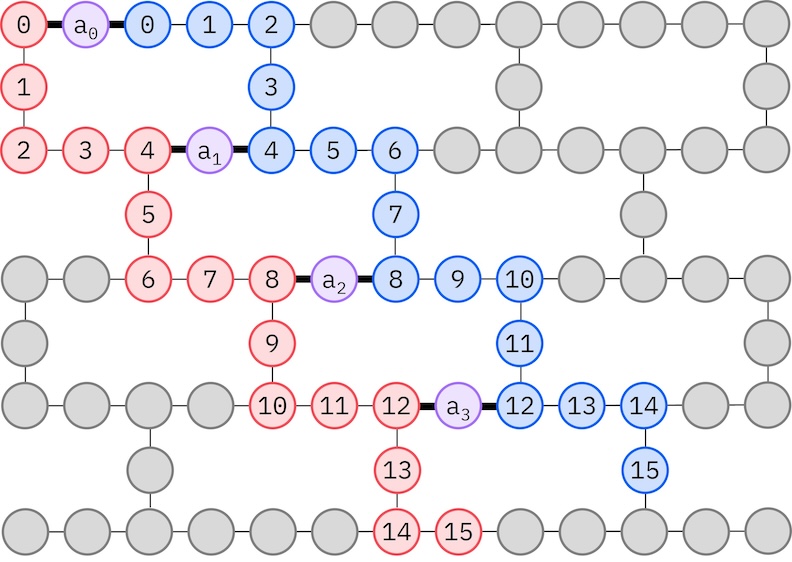
ターゲットのIBMハードウェアはヘビーヘックストポロジーを持つため、Qubit 相互作用の ジグザグ パターンを採用します。このパターンでは、同じスピンを持つ軌道（Qubit で表される）がライントポロジー（赤と青の円）で接続されており、ターゲットハードウェアのヘビーヘックス接続性によってジグザグ形状になります。また、ヘビーヘックストポロジーのため、異なるスピンの軌道は4番目ごとの軌道（0、4、8など）の間に接続があります（紫の円）。

lucj_ansatz

import ffsim
from qiskit import QuantumCircuit, QuantumRegister

n_reps = 1
alpha_alpha_indices = [(p, p + 1) for p in range(num_orbitals - 1)]
alpha_beta_indices = [(p, p) for p in range(0, num_orbitals, 4)]

ucj_op = ffsim.UCJOpSpinBalanced.from_t_amplitudes(
    t2=t2,
    t1=t1,
    n_reps=n_reps,
    interaction_pairs=(alpha_alpha_indices, alpha_beta_indices),
)

nelec = (num_elec_a, num_elec_b)

# create an empty quantum circuit
qubits = QuantumRegister(2 * num_orbitals, name="q")
circuit = QuantumCircuit(qubits)

# prepare Hartree-Fock state as the reference state and append it to the quantum circuit
circuit.append(ffsim.qiskit.PrepareHartreeFockJW(num_orbitals, nelec), qubits)

# apply the UCJ operator to the reference state
circuit.append(ffsim.qiskit.UCJOpSpinBalancedJW(ucj_op), qubits)
circuit.measure_all()

ステップ2：問題を最適化する

次に、ターゲットハードウェア向けに Circuit を最適化します。Circuit を最適化する前に、使用するハードウェアデバイスを選択する必要があります。実際のデバイスをエミュレートするために、qiskit_ibm_runtime の127 Qubit フェイク Backend を使用します。実際のQPUで実行する場合は、フェイク Backend を実際の Backend に置き換えてください。詳細については、Qiskit IBM Runtime ドキュメントを参照してください。

from qiskit_ibm_runtime.fake_provider import FakeSherbrooke

backend = FakeSherbrooke()

次に、アンザッツを最適化してハードウェア互換にするための以下の手順を推奨します。

ターゲットハードウェアから、上記のジグザグパターンに沿った物理 Qubit（initial_layout）を選択する。このパターンで Qubit を配置することで、ゲート数の少ない効率的なハードウェア互換 Circuit が得られます。
QiskitのTranspiler の generate_preset_pass_manager 関数を使用して、選択した backend と initial_layout でステージ付きパスマネージャを生成する。
ステージ付きパスマネージャの pre_init ステージを ffsim.qiskit.PRE_INIT に設定する。ffsim.qiskit.PRE_INIT には、ゲートを軌道回転に分解し、その後軌道回転をマージするQiskit Transpiler パスが含まれており、最終的な Circuit のゲート数が少なくなります。
Circuit 上でパスマネージャを実行する。

from qiskit.transpiler.preset_passmanagers import generate_preset_pass_manager

spin_a_layout = [0, 14, 18, 19, 20, 33, 39, 40, 41, 53, 60, 61, 62, 72, 81, 82]
spin_b_layout = [2, 3, 4, 15, 22, 23, 24, 34, 43, 44, 45, 54, 64, 65, 66, 73]
initial_layout = spin_a_layout + spin_b_layout

pass_manager = generate_preset_pass_manager(
    optimization_level=3, backend=backend, initial_layout=initial_layout
)

# without PRE_INIT passes
isa_circuit = pass_manager.run(circuit)
print(f"Gate counts (w/o pre-init passes): {isa_circuit.count_ops()}")

# with PRE_INIT passes
# We will use the circuit generated by this pass manager for hardware execution
pass_manager.pre_init = ffsim.qiskit.PRE_INIT
isa_circuit = pass_manager.run(circuit)
print(f"Gate counts (w/ pre-init passes): {isa_circuit.count_ops()}")

Gate counts (w/o pre-init passes): OrderedDict({'rz': 4420, 'sx': 3432, 'ecr': 1366, 'x': 239, 'measure': 32, 'barrier': 1})
Gate counts (w/ pre-init passes): OrderedDict({'rz': 2460, 'sx': 2156, 'ecr': 730, 'x': 71, 'measure': 32, 'barrier': 1})

ステップ3：実験を実行する

ハードウェア実行向けに Circuit を最適化した後、ターゲットハードウェアで実行して基底状態エネルギー推定のためのサンプルを収集する準備が整いました。Circuit は1つのみであるため、Qiskit Runtime のジョブ実行モードを使用して Circuit を実行します。

注：QPUで Circuit を実行するコードはコメントアウトし、ユーザーの参考のために残しています。このガイドでは実際のハードウェアでの実行の代わりに、一様分布から取得したランダムサンプルを生成します。

import numpy as np
from qiskit_addon_sqd.counts import generate_bit_array_uniform

# from qiskit_ibm_runtime import SamplerV2 as Sampler

# sampler = Sampler(mode=backend)
# job = sampler.run([isa_circuit], shots=10_000)
# primitive_result = job.result()
# pub_result = primitive_result[0]
# bit_array = pub_result.data.meas

rng = np.random.default_rng(24)
bit_array = generate_bit_array_uniform(10_000, num_orbitals * 2, rand_seed=rng)

ステップ4：結果を後処理する

ここで、diagonalize_fermionic_hamiltonian 関数を使用してSQDアルゴリズムを実行します。この関数の引数の説明については、APIドキュメントを参照してください。

SQDアドオンに含まれるソルバーは、PySCFの選択的CIの実装、具体的には pyscf.fci.selected_ci.kernel_fixed_space を使用します。以下の例では、含まれるソルバーを介してその関数にキーワード引数を渡す方法も示しています。ここでは max_cycle 引数を渡します。

from functools import partial

from qiskit_addon_sqd.fermion import SCIResult, diagonalize_fermionic_hamiltonian, solve_sci_batch

# SQD options
energy_tol = 1e-3
occupancies_tol = 1e-3
max_iterations = 5

# Eigenstate solver options
num_batches = 1
samples_per_batch = 300
symmetrize_spin = True
carryover_threshold = 1e-4
max_cycle = 200

# Pass options to the built-in eigensolver. If you just want to use the defaults,
# you can omit this step, in which case you would not specify the sci_solver argument
# in the call to diagonalize_fermionic_hamiltonian below.
sci_solver = partial(solve_sci_batch, spin_sq=0.0, max_cycle=max_cycle)

# List to capture intermediate results
result_history = []

def callback(results: list[SCIResult]):
    result_history.append(results)
    iteration = len(result_history)
    print(f"Iteration {iteration}")
    for i, result in enumerate(results):
        print(f"\tSubsample {i}")
        print(f"\t\tEnergy: {result.energy + nuclear_repulsion_energy}")
        print(f"\t\tSubspace dimension: {np.prod(result.sci_state.amplitudes.shape)}")

result = diagonalize_fermionic_hamiltonian(
    hcore,
    eri,
    bit_array,
    samples_per_batch=samples_per_batch,
    norb=num_orbitals,
    nelec=nelec,
    num_batches=num_batches,
    energy_tol=energy_tol,
    occupancies_tol=occupancies_tol,
    max_iterations=max_iterations,
    sci_solver=sci_solver,
    symmetrize_spin=symmetrize_spin,
    carryover_threshold=carryover_threshold,
    callback=callback,
    seed=rng,
)

Iteration 1
	Subsample 0
		Energy: -105.45358671756313
		Subspace dimension: 5476
Iteration 2
	Subsample 0
		Energy: -107.95172900082163
		Subspace dimension: 249001
Iteration 3
	Subsample 0
		Energy: -108.97460330369815
		Subspace dimension: 339889
Iteration 4
	Subsample 0
		Energy: -109.02739376648793
		Subspace dimension: 440896
Iteration 5
	Subsample 0
		Energy: -109.030972328451
		Subspace dimension: 597529

次に、結果をプロットします。

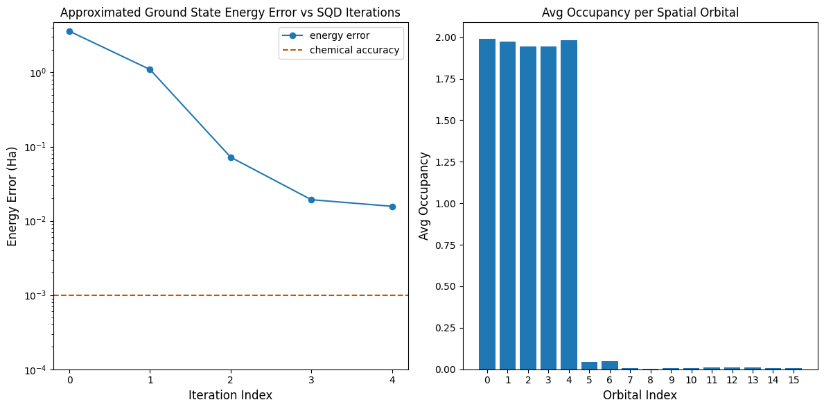
最初のプロットは、数回のイテレーション後に基底状態エネルギーを ~16 mH 以内で推定していることを示しています（化学精度は通常 1 kcal/mol $\approx$ 1.6 mH と定義されています）。このデモの量子サンプルは純粋なノイズであることを思い出してください。ここでのシグナルは、電子構造と分子ハミルトニアンに関する事前知識から得られています。

2番目のプロットは、最終イテレーション後の各空間軌道の平均占有率を示しています。スピンアップおよびスピンダウン電子が、解の中で高い確率で最初の5つの軌道を占有していることがわかります。

import matplotlib.pyplot as plt

# Data for energies plot
x1 = range(len(result_history))
min_e = [
    min(result, key=lambda res: res.energy).energy + nuclear_repulsion_energy
    for result in result_history
]
e_diff = [abs(e - exact_energy) for e in min_e]
yt1 = [1.0, 1e-1, 1e-2, 1e-3, 1e-4]

# Chemical accuracy (+/- 1 milli-Hartree)
chem_accuracy = 0.001

# Data for avg spatial orbital occupancy
y2 = np.sum(result.orbital_occupancies, axis=0)
x2 = range(len(y2))

fig, axs = plt.subplots(1, 2, figsize=(12, 6))

# Plot energies
axs[0].plot(x1, e_diff, label="energy error", marker="o")
axs[0].set_xticks(x1)
axs[0].set_xticklabels(x1)
axs[0].set_yticks(yt1)
axs[0].set_yticklabels(yt1)
axs[0].set_yscale("log")
axs[0].set_ylim(1e-4)
axs[0].axhline(y=chem_accuracy, color="#BF5700", linestyle="--", label="chemical accuracy")
axs[0].set_title("Approximated Ground State Energy Error vs SQD Iterations")
axs[0].set_xlabel("Iteration Index", fontdict={"fontsize": 12})
axs[0].set_ylabel("Energy Error (Ha)", fontdict={"fontsize": 12})
axs[0].legend()

# Plot orbital occupancy
axs[1].bar(x2, y2, width=0.8)
axs[1].set_xticks(x2)
axs[1].set_xticklabels(x2)
axs[1].set_title("Avg Occupancy per Spatial Orbital")
axs[1].set_xlabel("Orbital Index", fontdict={"fontsize": 12})
axs[1].set_ylabel("Avg Occupancy", fontdict={"fontsize": 12})

print(f"Exact energy: {exact_energy:.5f} Ha")
print(f"SQD energy: {min_e[-1]:.5f} Ha")
print(f"Absolute error: {e_diff[-1]:.5f} Ha")
plt.tight_layout()
plt.show()

Exact energy: -109.04667 Ha
SQD energy: -109.03097 Ha
Absolute error: 0.01570 Ha

Plot output

ステップ1：問題を量子 Circuit にマッピングする​

ステップ2：問題を最適化する​

ステップ3：実験を実行する​

ステップ4：結果を後処理する​

ステップ1：問題を量子 Circuit にマッピングする

ステップ2：問題を最適化する

ステップ3：実験を実行する

ステップ4：結果を後処理する