オペレーター逆伝播による回路の深さの削減

オペレーター逆伝播（operator backpropagation）は、量子回路の末尾から演算をパウリ演算子に吸収する手法です。一般に、演算子の項数が増える代わりに回路の深さを削減できます。目標は、演算子が大きくなりすぎないようにしながら、できるだけ多くの回路を逆伝播させることです。

演算子が大きくなりすぎることを防ぎながら、回路への逆伝播をより深く行う方法の一つは、演算子に追加する代わりに、係数が小さい項を切り捨てることです。項の切り捨てにより、実行する量子回路の数を減らすことができますが、切り捨てた項の係数の大きさに比例した誤差が最終的な期待値の計算に生じます。 このチュートリアルでは、オペレーター逆伝播を使用してハイゼンベルク・スピン鎖の量子ダイナミクスをシミュレートするための Qiskit パターン を実装します。

• ステップ 1: 量子問題へのマッピング
  • 時間発展したハミルトニアンを量子回路にマッピングする
• ステップ 2: 問題の最適化
  • 回路をスライスに分割する
  • 回路からスライスをパウリ・オブザーバブルに逆伝播させる
  • 残りのスライスを単一の回路にまとめる
  • Backend 向けに回路をトランスパイルする
• ステップ 3: 実験の実行
  • このノートブックでは簡略化のため、StatevectorEstimator を使用して、削減された回路と拡張されたオブザーバブルで期待値を計算する
• ステップ 4: 結果の再構成
  • 該当なし

注: Qiskit では、レイヤー を、すべての Qubit にわたる回路の深さ 1 のパーティションとして定義しています。このパッケージでは、任意の深さのレイヤーを表す用語として スライス を使用しています。qiskit_addon_obp.backpropagate 関数はスライス全体を一度に逆伝播するように設計されているため、量子回路のスライス方法の選択は、逆伝播が特定の問題に対してどの程度有効かに大きな影響を与えます。スライス については以下で詳しく説明します。

ステップ 1: 量子問題へのマッピング

量子ハイゼンベルク模型の時間発展を量子実験にマッピングする

qiskit_addon_utils パッケージは、さまざまな目的に対応した再利用可能な機能を提供しています。

その qiskit_addon_utils.problem_generators モジュールは、指定した結合グラフ上のハイゼンベルク型ハミルトニアンを生成する関数を提供します。 このグラフには rustworkx.PyGraph または CouplingMap のいずれかを使用でき、Qiskit 中心のワークフローで簡単に活用できます。

以下では、まずヘビー・ヘックス型の CouplingMap を生成し、そこから 10 Qubit の線形チェーンを切り出します。なお、この新しい reduced_coupling_map のインデックスは再びゼロベースになります。

# Added by doQumentation — required packages for this notebook
!pip install -q numpy qiskit qiskit-addon-obp qiskit-addon-utils qiskit-ibm-runtime rustworkx

from qiskit.transpiler import CouplingMap

coupling_map = CouplingMap.from_heavy_hex(3, bidirectional=False)

# Choose a 10-qubit linear chain on this coupling map
reduced_coupling_map = coupling_map.reduce([0, 13, 1, 14, 10, 16, 5, 12, 8, 18])

from rustworkx.visualization import graphviz_draw

graphviz_draw(reduced_coupling_map.graph, method="circo")

次に、ハイゼンベルク XYZ ハミルトニアンをモデル化するパウリ演算子を生成します。

J_{y} \sigma_j^{y} \sigma_{k}^{y} + J_{z} \sigma_j^{z} \sigma_{k}^{z}) + \sum_{j\in V} (h_{x} \sigma_j^{x} + h_{y} \sigma_j^{y} + h_{z} \sigma_j^{z})$$ ここで $G(V,E)$ は提供された結合マップのグラフです。 ```python import numpy as np from qiskit_addon_utils.problem_generators import generate_xyz_hamiltonian # Get a qubit operator describing the Heisenberg XYZ model hamiltonian = generate_xyz_hamiltonian( reduced_coupling_map, coupling_constants=(np.pi / 8, np.pi / 4, np.pi / 2), ext_magnetic_field=(np.pi / 3, np.pi / 6, np.pi / 9), ) print(hamiltonian) ``` ```text SparsePauliOp(['IIIIIIIXXI', 'IIIIIIIYYI', 'IIIIIIIZZI', 'IIIIIXXIII', 'IIIIIYYIII', 'IIIIIZZIII', 'IIIXXIIIII', 'IIIYYIIIII', 'IIIZZIIIII', 'IXXIIIIIII', 'IYYIIIIIII', 'IZZIIIIIII', 'IIIIIIIIXX', 'IIIIIIIIYY', 'IIIIIIIIZZ', 'IIIIIIXXII', 'IIIIIIYYII', 'IIIIIIZZII', 'IIIIXXIIII', 'IIIIYYIIII', 'IIIIZZIIII', 'IIXXIIIIII', 'IIYYIIIIII', 'IIZZIIIIII', 'XXIIIIIIII', 'YYIIIIIIII', 'ZZIIIIIIII', 'IIIIIIIIIX', 'IIIIIIIIIY', 'IIIIIIIIIZ', 'IIIIIIIIXI', 'IIIIIIIIYI', 'IIIIIIIIZI', 'IIIIIIIXII', 'IIIIIIIYII', 'IIIIIIIZII', 'IIIIIIXIII', 'IIIIIIYIII', 'IIIIIIZIII', 'IIIIIXIIII', 'IIIIIYIIII', 'IIIIIZIIII', 'IIIIXIIIII', 'IIIIYIIIII', 'IIIIZIIIII', 'IIIXIIIIII', 'IIIYIIIIII', 'IIIZIIIIII', 'IIXIIIIIII', 'IIYIIIIIII', 'IIZIIIIIII', 'IXIIIIIIII', 'IYIIIIIIII', 'IZIIIIIIII', 'XIIIIIIIII', 'YIIIIIIIII', 'ZIIIIIIIII'], coeffs=[0.39269908+0.j, 0.78539816+0.j, 1.57079633+0.j, 0.39269908+0.j, 0.78539816+0.j, 1.57079633+0.j, 0.39269908+0.j, 0.78539816+0.j, 1.57079633+0.j, 0.39269908+0.j, 0.78539816+0.j, 1.57079633+0.j, 0.39269908+0.j, 0.78539816+0.j, 1.57079633+0.j, 0.39269908+0.j, 0.78539816+0.j, 1.57079633+0.j, 0.39269908+0.j, 0.78539816+0.j, 1.57079633+0.j, 0.39269908+0.j, 0.78539816+0.j, 1.57079633+0.j, 0.39269908+0.j, 0.78539816+0.j, 1.57079633+0.j, 1.04719755+0.j, 0.52359878+0.j, 0.34906585+0.j, 1.04719755+0.j, 0.52359878+0.j, 0.34906585+0.j, 1.04719755+0.j, 0.52359878+0.j, 0.34906585+0.j, 1.04719755+0.j, 0.52359878+0.j, 0.34906585+0.j, 1.04719755+0.j, 0.52359878+0.j, 0.34906585+0.j, 1.04719755+0.j, 0.52359878+0.j, 0.34906585+0.j, 1.04719755+0.j, 0.52359878+0.j, 0.34906585+0.j, 1.04719755+0.j, 0.52359878+0.j, 0.34906585+0.j, 1.04719755+0.j, 0.52359878+0.j, 0.34906585+0.j, 1.04719755+0.j, 0.52359878+0.j, 0.34906585+0.j]) ``` Qubit 演算子から、その時間発展をモデル化する量子回路を生成できます。 ここでも [qiskit_addon_utils.problem_generators](https://qiskit.github.io/qiskit-addon-utils/stubs/qiskit_addon_utils.problem_generators.html) モジュールが役立つ関数を提供しています。 ```python from qiskit.synthesis import LieTrotter from qiskit_addon_utils.problem_generators import generate_time_evolution_circuit circuit = generate_time_evolution_circuit( hamiltonian, time=0.2, synthesis=LieTrotter(reps=2), ) circuit.draw("mpl", style="iqp", scale=0.6) ``` 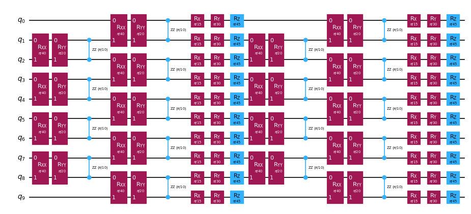 ## ステップ 2: 問題の最適化 \{#step-2-optimize-the-problem} ### 逆伝播するための回路スライスを作成する \{#create-circuit-slices-to-backpropagate} ``backpropagate`` 関数はスライス全体を一度に逆伝播させることを覚えておいてください。そのため、スライス方法の選択は、逆伝播が特定の問題に対してどの程度有効かに影響を与えます。ここでは、[slice_by_gate_types](https://qiskit.github.io/qiskit-addon-utils/stubs/qiskit_addon_utils.slicing.slice_by_gate_types.html) 関数を使用して、同じ種類の Gate をスライスにグループ化します。 回路スライシングの詳細な説明については、[qiskit-addon-utils](https://qiskit.github.io/qiskit-addon-utils/index.html) パッケージの [ハウツー・ガイド](https://qiskit.github.io/qiskit-addon-utils/how_tos/create_circuit_slices.html) を参照してください。 ```python from qiskit_addon_utils.slicing import slice_by_gate_types slices = slice_by_gate_types(circuit) print(f"Separated the circuit into {len(slices)} slices.") ``` ```text Separated the circuit into 18 slices. ``` ### 逆伝播中に演算子が成長できる大きさを制限する \{#constrain-how-large-the-operator-may-grow-during-backpropagation} 逆伝播中、演算子の項数は一般に $4^N$ に近づくように急速に増加します。ここで $N$ は Qubit の数です。演算子のサイズは、``backpropagate`` 関数の ``operator_budget`` キーワード引数に [OperatorBudget](https://qiskit.github.io/qiskit-addon-obp/stubs/qiskit_addon_obp.utils.simplify.OperatorBudget.html) インスタンスを指定することで制限できます。 ここでは、演算子内の Qubit ごとに可換なパウリ・グループの数が 8 を超えた時点で逆伝播を停止するように指定します。 ```python from qiskit_addon_obp.utils.simplify import OperatorBudget op_budget = OperatorBudget(max_qwc_groups=8) ``` ### 回路からスライスを逆伝播させる \{#backpropagate-slices-from-the-circuit} まず、Qubit 0 上のパウリ Z オブザーバブルを指定し、オブザーバブルの項が 8 つ以下の Qubit ごとに可換なパウリ・グループにまとめられなくなるまで、時間発展回路からスライスを逆伝播させます。 以下では、7 つのスライスを逆伝播させましたが、割り当てられた 8 つのパウリ・グループのうち 6 つしか使用していないことがわかります。これは、もう 1 つスライスを逆伝播させるとパウリ・グループの数が 8 を超えることを意味します。返されたメタデータを確認することで、これが事実であることを検証できます。 ```python from qiskit.quantum_info import SparsePauliOp from qiskit_addon_obp import backpropagate from qiskit_addon_utils.slicing import combine_slices # Specify a single-qubit observable observable = SparsePauliOp("IIIIIIIIIZ") # Backpropagate slices onto the observable bp_obs, remaining_slices, metadata = backpropagate(observable, slices, operator_budget=op_budget) # Recombine the slices remaining after backpropagation bp_circuit = combine_slices(remaining_slices, include_barriers=True) print(f"Backpropagated {metadata.num_backpropagated_slices} slices.") print( f"New observable has {len(bp_obs.paulis)} terms, which can be combined into {len(bp_obs.group_commuting(qubit_wise=True))} groups." ) print( f"Note that backpropagating one more slice would result in {metadata.backpropagation_history[-1].num_paulis[0]} terms " f"across {metadata.backpropagation_history[-1].num_qwc_groups} groups." ) print("The remaining circuit after backpropagation looks as follows:") bp_circuit.draw("mpl", scale=0.6) ``` ```text Backpropagated 7 slices. New observable has 18 terms, which can be combined into 8 groups. Note that backpropagating one more slice would result in 27 terms across 12 groups. The remaining circuit after backpropagation looks as follows: ``` 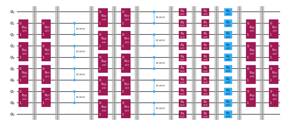 次に、出力されるオブザーバブルのサイズに対して同じ制約を用いて同じ問題を指定します。ただし今回は、[setup_budet](https://qiskit.github.io/qiskit-addon-obp/stubs/qiskit_addon_obp.utils.truncating.setup_budget.html) 関数を使用して各スライスに誤差バジェットを割り当てます。各スライスから係数が小さいパウリ・タームが誤差バジェットが満たされるまで切り捨てられ、余ったバジェットは次のスライスのバジェットに追加されます。 この切り捨てを有効にするには、以下のように誤差バジェットを設定する必要があります。 ```python from qiskit_addon_obp.utils.truncating import setup_budget truncation_error_budget = setup_budget(max_error_per_slice=0.005) ``` 切り捨てのためにスライスごとに `5e-3` の誤差を割り当てることで、オブザーバブル内の可換なパウリ・グループの元の上限 8 を維持しながら、回路からさらに 3 つのスライスを除去できることに注意してください。デフォルトでは、`backpropagate` は切り捨てられた係数の L1 ノルムを使用して、切り捨てによって生じる合計誤差を制限します。その他のオプションについては、[p_norm の指定に関するハウツー・ガイド](https://qiskit.github.io/qiskit-addon-obp/how_tos/bound_error_using_p_norm.html) を参照してください。 10 スライスを逆伝播させたこの特定の例では、合計切り捨て誤差は ``(5e-3 error/slice) * (10 slices) = 5e-2`` を超えてはなりません。 スライス間の誤差バジェットの配分に関する詳細な説明については、[このハウツー・ガイド](https://qiskit.github.io/qiskit-addon-obp/how_tos/truncate_operator_terms.html) を参照してください。 ```python # Run the same experiment but truncate observable terms with small coefficients bp_obs_trunc, remaining_slices_trunc, metadata = backpropagate( observable, slices, operator_budget=op_budget, truncation_error_budget=truncation_error_budget ) # Recombine the slices remaining after backpropagation bp_circuit_trunc = combine_slices(remaining_slices_trunc, include_barriers=True) print(f"Backpropagated {metadata.num_backpropagated_slices} slices.") print( f"New observable has {len(bp_obs_trunc.paulis)} terms, which can be combined into {len(bp_obs_trunc.group_commuting(qubit_wise=True))} groups.\n" f"After truncation, the error in our observable is bounded by {metadata.accumulated_error(0):.3e}" ) print( f"Note that backpropagating one more slice would result in {metadata.backpropagation_history[-1].num_paulis[0]} terms " f"across {metadata.backpropagation_history[-1].num_qwc_groups} groups." ) print("The remaining circuit after backpropagation looks as follows:") bp_circuit_trunc.draw("mpl", scale=0.6) ``` ```text Backpropagated 10 slices. New observable has 19 terms, which can be combined into 8 groups. After truncation, the error in our observable is bounded by 4.933e-02 Note that backpropagating one more slice would result in 27 terms across 13 groups. The remaining circuit after backpropagation looks as follows: ``` 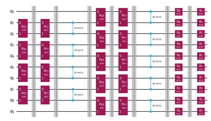 ### 削減されたアンザッツと拡張されたオブザーバブルが得られたので、実験を Backend にトランスパイルできます。 \{#now-that-we-have-our-reduced-ansatze-and-expanded-observables-we-can-transpile-our-experiments-to-the-backend} ここでは、[qiskit-ibm-runtime](https://quantum.cloud.ibm.com/docs/api/qiskit-ibm-runtime) の 14 Qubit の [FakeMelbourneV2](https://quantum.cloud.ibm.com/docs/api/qiskit-ibm-runtime/fake-provider-fake-melbourne-v2) を使用して、QPU Backend へのトランスパイル方法を説明します。 ```python from qiskit.transpiler.preset_passmanagers import generate_preset_pass_manager from qiskit_ibm_runtime.fake_provider import FakeMelbourneV2 # Specify a backend and a pass manager for transpilation backend = FakeMelbourneV2() pm = generate_preset_pass_manager(backend=backend, optimization_level=1) # Transpile original experiment circuit_isa = pm.run(circuit) observable_isa = observable.apply_layout(circuit_isa.layout) # Transpile backpropagated experiment bp_circuit_isa = pm.run(bp_circuit) bp_obs_isa = bp_obs.apply_layout(bp_circuit_isa.layout) # Transpile the backpropagated experiment with truncated observable terms bp_circuit_trunc_isa = pm.run(bp_circuit_trunc) bp_obs_trunc_isa = bp_obs_trunc.apply_layout(bp_circuit_trunc_isa.layout) ``` ## ステップ 3: 量子実験の実行 \{#step-3-execute-quantum-experiments} ### 期待値を計算する \{#calculate-expectation-value} 最後に、ノイズのない [StatevectorEstimator](https://quantum.cloud.ibm.com/docs/api/qiskit/qiskit.primitives.StatevectorEstimator) を使用して、逆伝播した実験を実行し、完全な実験と比較できます。切り捨てなしの逆伝播期待値は、数値精度の範囲内で正確な値と等しいことがわかります。 切り捨てられた項を持つ演算子の期待値には ``1e-4`` オーダーの誤差がありますが、これは想定される許容範囲内です。 **注:** 切り捨てが出力に与える影響を示すために、状態ベクトルベースの ``Estimator`` プリミティブを使用しています。ステップ 2 でトランスパイルした Backend 上で実行するには、``qiskit-ibm-runtime`` から [EstimatorV2](https://quantum.cloud.ibm.com/docs/api/qiskit-ibm-runtime/estimator-v2) をインポートし、コンストラクターに Backend インスタンスを渡します。 ```python from qiskit.primitives import StatevectorEstimator as Estimator estimator = Estimator() # Run the experiments using Estimator primitive result_exact = estimator.run([(circuit_isa, observable_isa)]).result()[0].data.evs.item() result_bp = estimator.run([(bp_circuit_isa, bp_obs_isa)]).result()[0].data.evs.item() result_bp_trunc = ( estimator.run([(bp_circuit_trunc_isa, bp_obs_trunc_isa)]).result()[0].data.evs.item() ) print(f"Exact expectation value: {result_exact}") print(f"Backpropagated expectation value: {result_bp}") print(f"Backpropagated expectation value with truncation: {result_bp_trunc}") print(f" - Expected Error for truncated observable: {metadata.accumulated_error(0):.3e}") print(f" - Observed Error for truncated observable: {abs(result_exact - result_bp_trunc):.3e}") ``` ```text Exact expectation value: 0.8854160687717507 Backpropagated expectation value: 0.8854160687717532 Backpropagated expectation value with truncation: 0.8850236647156059 - Expected Error for truncated observable: 4.933e-02 - Observed Error for truncated observable: 3.924e-04 ``` <TutorialFeedback />