Gate Cutting による Circuit 深度の削減

このチュートリアルでは、遠距離の Gate を切断することで Circuit の深度を削減し、ルーティングによって導入されるスワップ Gate を回避します。

ここでは、以下の Qiskit パターン の手順を実行します：

• Step 1: 問題を量子 Circuit と演算子にマッピングする：
  • ハミルトニアンを量子 Circuit にマッピングします。
• Step 2: 対象ハードウェア向けに最適化する [カッティング・アドオンを使用]：
  • Circuit と観測量を切断します。
  • ハードウェア向けにサブ実験をトランスパイルします。
• Step 3: 対象ハードウェアで実行する：
  • Step 2 で得られたサブ実験を Sampler プリミティブを使って実行します。
• Step 4: 結果を後処理する [カッティング・アドオンを使用]：
  • Step 3 の結果を組み合わせて、対象となる観測量の期待値を再構成します。

Step 1: マッピング

Backend で実行する Circuit を作成する

# Added by doQumentation — required packages for this notebook
!pip install -q numpy qiskit qiskit-addon-cutting qiskit-aer qiskit-ibm-runtime

from qiskit.circuit.library import efficient_su2

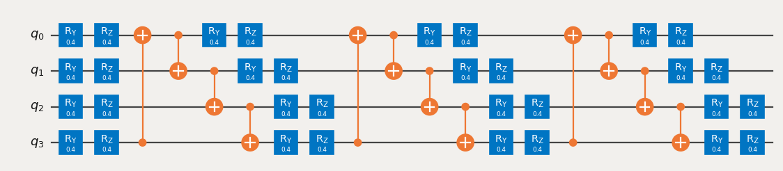
circuit = efficient_su2(num_qubits=4, entanglement="circular")
circuit.assign_parameters([0.4] * len(circuit.parameters), inplace=True)
circuit.draw("mpl", scale=0.8)

観測量を指定する

from qiskit.quantum_info import SparsePauliOp

observable = SparsePauliOp(["ZZII", "IZZI", "-IIZZ", "XIXI", "ZIZZ", "IXIX"])

Step 2: 最適化

Backend を指定する

フェイク Backend または Qiskit Runtime のハードウェア Backend を指定できます。

from qiskit_ibm_runtime.fake_provider import FakeManilaV2

backend = FakeManilaV2()

Circuit をトランスパイルし、スワップを可視化して深度を確認する

Qubit 3 と 0 の間の Gate を実行するために 2 回のスワップが必要となり、さらに Qubit を初期位置に戻すためにもう 2 回のスワップが必要となるレイアウトを選択します。

from qiskit.transpiler import generate_preset_pass_manager

pass_manager = generate_preset_pass_manager(
    optimization_level=1, backend=backend, initial_layout=[0, 1, 2, 3]
)

transpiled_qc = pass_manager.run(circuit)
print(f"Transpiled circuit depth: {transpiled_qc.depth(lambda x: len(x.qubits) >= 2)}")

Transpiled circuit depth: 30

transpiled_qc.draw("mpl", scale=0.4, idle_wires=False, fold=-1)

インデックスを指定して遠距離 Gate を TwoQubitQPDGate に置き換える

cut_gates は、指定されたインデックスにある Gate を TwoQubitQPDGate に置き換え、各 Gate 分解に対する QPDBasis インスタンスのリストも返します。

from qiskit_addon_cutting import cut_gates

# Find the indices of the distant gates
cut_indices = [
    i
    for i, instruction in enumerate(circuit.data)
    if {circuit.find_bit(q)[0] for q in instruction.qubits} == {0, 3}
]

# Decompose distant CNOTs into TwoQubitQPDGate instances
qpd_circuit, bases = cut_gates(circuit, cut_indices)

qpd_circuit.draw("mpl", scale=0.8)

Backend で実行するサブ実験を生成する

generate_cutting_experiments は、TwoQubitQPDGate インスタンスを含む Circuit と、PauliList としての観測量を受け取ります。

フルサイズの Circuit の期待値をシミュレートするために、分解された Gate の結合準確率分布から多数のサブ実験が生成され、1 つ以上の Backend で実行されます。分布からのサンプル数は num_samples で制御され、一意のサンプルごとに 1 つの結合係数が与えられます。係数の計算方法の詳細については、説明資料 を参照してください。

注意： generate_cutting_experiments の observables キーワード引数の型は PauliList です。観測量の項の係数と位相は、問題の分解およびサブ実験の実行中は無視されます。期待値の再構成時に再適用することができます。

import numpy as np
from qiskit_addon_cutting import generate_cutting_experiments

# Generate the subexperiments and sampling coefficients
subexperiments, coefficients = generate_cutting_experiments(
    circuits=qpd_circuit, observables=observable.paulis, num_samples=np.inf
)

選択した切断のサンプリング・オーバーヘッドを計算する

ここでは 3 つの CNOT Gate を切断しており、サンプリング・オーバーヘッドは $9^3$ になります。

Circuit カッティングによるサンプリング・オーバーヘッドの詳細については、説明資料 を参照してください。

print(f"Sampling overhead: {np.prod([basis.overhead for basis in bases])}")

Sampling overhead: 729.0

遠距離 Gate を切断した後の QPD サブ実験がより浅くなることを示す

以下は、QPD Circuit から生成された任意に選択されたサブ実験の例です。その深度は半分以上削減されています。より深い Circuit の期待値を再構成するためには、これらの確率的サブ実験を多数生成して評価する必要があります。

# Transpile the decomposed circuit to the same layout
transpiled_qpd_circuit = pass_manager.run(subexperiments[100])

print(
    f"Original circuit depth after transpile: {transpiled_qc.depth(lambda x: len(x.qubits) >= 2)}"
)
print(
    f"QPD subexperiment depth after transpile: {transpiled_qpd_circuit.depth(lambda x: len(x.qubits) >= 2)}"
)
transpiled_qpd_circuit.draw("mpl", scale=0.8, idle_wires=False, fold=-1)

Original circuit depth after transpile: 30
QPD subexperiment depth after transpile: 7

Backend 向けにサブ実験を準備する

# Transpile the subeperiments to the backend's instruction set architecture (ISA)
isa_subexperiments = pass_manager.run(subexperiments)

Step 3: 実行

Qiskit Runtime Sampler プリミティブを使ってサブ実験を実行する

from qiskit_ibm_runtime import SamplerV2

# Set up the Qiskit Runtime Sampler primitive.  For a fake backend, this will use a local simulator.
sampler = SamplerV2(backend)

# Submit the subexperiments
job = sampler.run(isa_subexperiments)

# Retrieve the results
results = job.result()

Step 4: 後処理

期待値を再構成する

各観測量の項の期待値を再構成し、それらを組み合わせて元の観測量の期待値を再構成します。

from qiskit_addon_cutting import reconstruct_expectation_values

reconstructed_expval_terms = reconstruct_expectation_values(
    results,
    coefficients,
    observable.paulis,
)
# Reconstruct final expectation value
reconstructed_expval = np.dot(reconstructed_expval_terms, observable.coeffs)

再構成した期待値を元の Circuit と観測量の正確な期待値と比較する

from qiskit_aer.primitives import EstimatorV2

estimator = EstimatorV2()
exact_expval = estimator.run([(circuit, observable)]).result()[0].data.evs
print(f"Reconstructed expectation value: {np.real(np.round(reconstructed_expval, 8))}")
print(f"Exact expectation value: {np.round(exact_expval, 8)}")
print(f"Error in estimation: {np.real(np.round(reconstructed_expval-exact_expval, 8))}")
print(
    f"Relative error in estimation: {np.real(np.round((reconstructed_expval-exact_expval) / exact_expval, 8))}"
)

Reconstructed expectation value: 0.44018555
Exact expectation value: 0.50497603
Error in estimation: -0.06479049
Relative error in estimation: -0.12830408