量子フーリエ変換

この「Qiskit in Classrooms」モジュールを使用するには、以下のパッケージがインストールされた Python 環境が必要です：

• qiskit v2.1.0 以降
• qiskit-ibm-runtime v0.40.1 以降
• qiskit-aer v0.17.0 以降
• qiskit.visualization
• numpy
• pylatexenc

上記パッケージのセットアップとインストールについては、Qiskit のインストールガイドを参照してください。 実際の量子コンピューターでジョブを実行するには、IBM Cloud アカウントのセットアップガイドの手順に従って IBM Quantum® のアカウントを作成する必要があります。

このモジュールはテスト済みで、QPU 時間を 13 秒使用しました。これはあくまで目安であり、実際の使用量は異なる場合があります。

# Added by doQumentation — required packages for this notebook
!pip install -q numpy qiskit qiskit-aer qiskit-ibm-runtime

# Uncomment and modify this line as needed to install dependencies
#!pip install 'qiskit>=2.1.0' 'qiskit-ibm-runtime>=0.40.1' 'qiskit-aer>=0.17.0' 'numpy' 'pylatexenc'

はじめに

フーリエ変換は、数学、物理学、信号処理、データ圧縮をはじめとする無数の分野で広く活用されている手法です。量子版のフーリエ変換、すなわち「量子フーリエ変換」は、最も重要な量子アルゴリズムの一部の基盤となっています。

本日は、古典的なフーリエ変換のおさらいをしたうえで、量子コンピューター上での量子フーリエ変換の実装方法について説明します。次に、量子フーリエ変換を応用した「位相推定アルゴリズム」についても解説します。量子位相推定は、量子コンピューティングの「最高傑作」とも呼ばれる Shor の素因数分解アルゴリズムのサブルーチンです。このモジュールは Shor のアルゴリズム全体を扱う別のモジュールへの足がかりとなっていますが、単体としても完結した内容を目指しています。量子フーリエ変換は、それ自体としても魅力的かつ有用なアルゴリズムです！

古典的フーリエ変換

量子フーリエ変換に踏み込む前に、まず古典版のフーリエ変換を振り返りましょう。フーリエ変換は、ある「基底」から別の基底へと変換する手法です。二つの基底は、同じ問題を異なる視点から見たものと考えることができます。どちらも関数を表現する有効な方法ですが、問題によってどちらか一方がより明快な場合があります。フーリエ変換によって結ばれる基底の組の例としては、位置と運動量、時間と周波数などが挙げられます。

では、フーリエ変換を使って、オーディオ波形からどの音が演奏されているかを識別する例を見てみましょう。通常、波形は時間基底で表現されます。つまり、波の振幅が時間の関数として表されます。

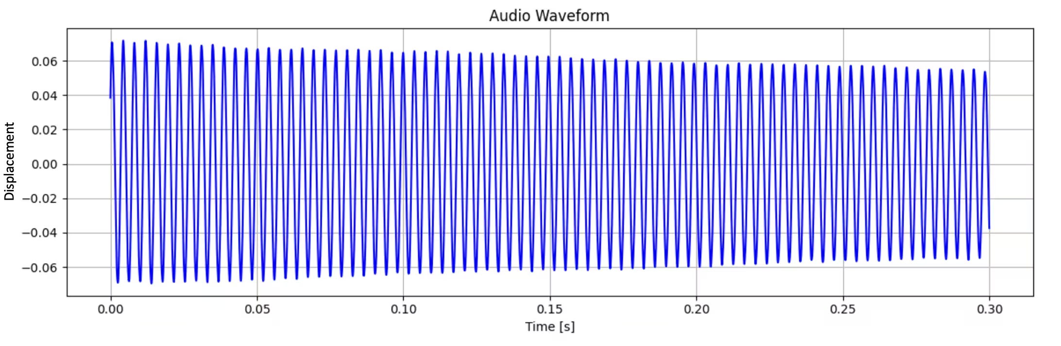
この波形をフーリエ変換することで、時間基底から周波数基底へ変換できます：

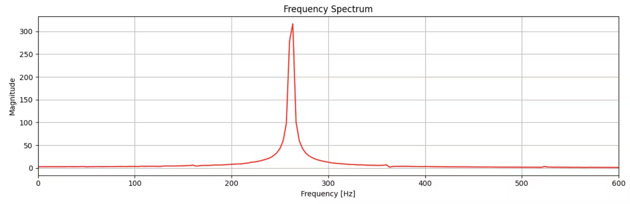
周波数基底では、約 260 Hz に明確なピークを確認できます。これはミドル C（中央のド）です！

フーリエ変換なしにミドル C が演奏されていることを判断できたかもしれませんが、複数の音が同時に演奏されている場合はどうでしょうか？時間基底でプロットすると、波形はより複雑になります：

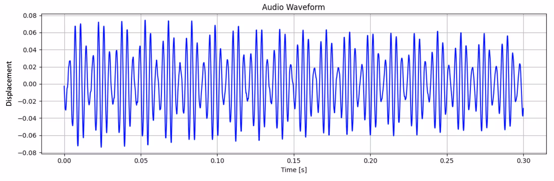
しかし、周波数スペクトルでは三つのピークがはっきりと識別されます：

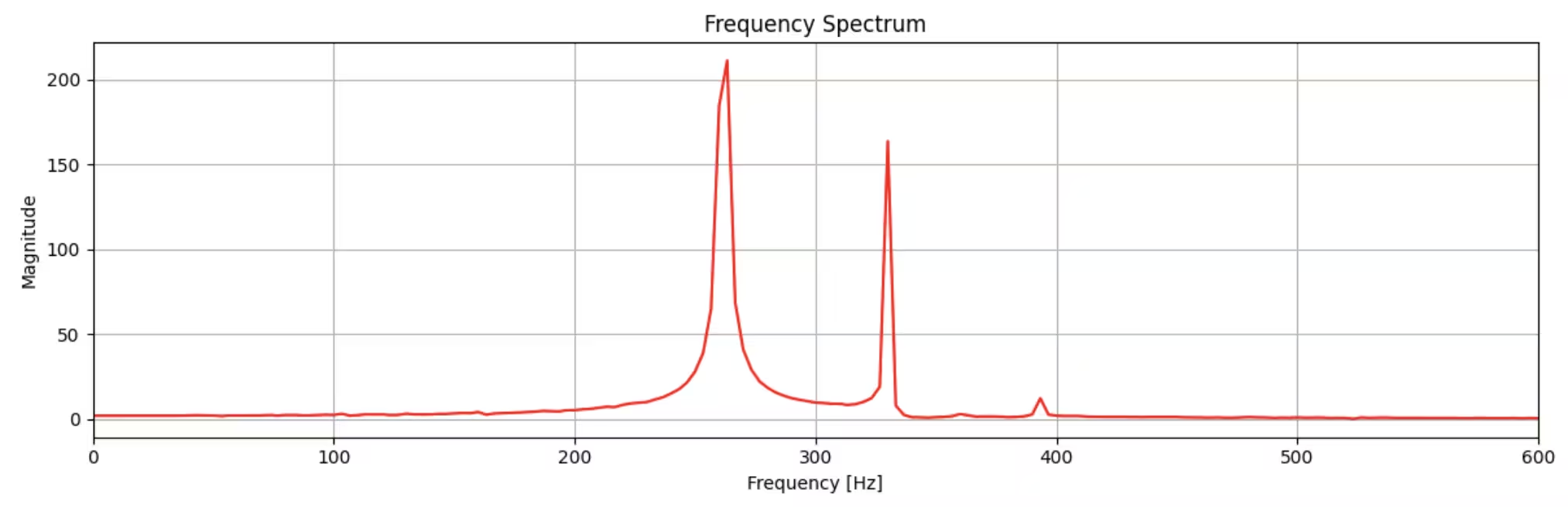
これは C メジャーコードで、ド・ミ・ソの音が演奏されていました。

このようなフーリエ解析を用いることで、あらゆる複雑な信号から周波数成分を抽出することができます。

離散フーリエ変換

フーリエ変換は、さまざまな信号処理アプリケーションで役立ちます。しかし、上述の音楽の例を含む多くの実世界のアプリケーションでは、連続関数ではなく、$N$ 個のデータ点からなる離散的な集合を変換する必要があります。この場合に使われるのが「離散フーリエ変換」（DFT）です。離散フーリエ変換（DFT）は、ベクトル $(x_0, ..., x_{N-1})$ に作用し、次の式に従ってベクトル $(y_0, ..., y_{N-1})$ へ写像します：

$y_k = \frac{1}{\sqrt{N}}\sum_{j=0}^{N-1}x_j\omega_N^{jk}$

ここで $\omega_N^{jk} = e^{2\pi i \frac{jk}{N}}$ とします。（指数部分に負符号が付く別の表記法もあるため、DFT の式を見かけた際は注意してください。）$e^{2\pi i \frac{jk}{N}}$ は周期 $\frac{N}{k}$ の周期関数であることを思い出してください。つまり、この関数との積を取ることで、フーリエ変換は本質的に離散関数 $\{x_{j}\}$ を、それぞれ周期 $\frac{N}{k}$ を持つ周期関数の線形結合に分解する操作となっています。

量子フーリエ変換

ここまでで、フーリエ変換がある関数を新しい「基底関数」の線形結合として表現するために使われることを見てきました。量子ビット状態においても、基底変換は日常的に行われます。たとえば、単一 Qubit の状態 $|\psi\rangle$ は、基底状態 $|0\rangle$ と $|1\rangle$ からなる計算基底で $|\psi\rangle = c_0 |0\rangle + c_1 |1\rangle$ と表すことも、基底状態 $|+\rangle = \frac{1}{\sqrt{2}} (|0\rangle + |1\rangle)$ と $|-\rangle = \frac{1}{\sqrt{2}} (|0\rangle - |1\rangle)$ からなる $X$ 基底で $|\psi\rangle = c_+ |+\rangle + c_- |-\rangle$ と表すこともできます。どちらも等しく有効な表現ですが、解こうとする問題の種類によってどちらか一方がより自然な場合があります。

Qubit 状態はフーリエ基底でも表現できます。この場合、状態は通常の計算基底状態 $|x\rangle$ ではなく、フーリエ基底状態 $|\phi_y\rangle$ の線形結合で表されます。これを行うには、量子フーリエ変換（QFT）を適用する必要があります：

$| \phi_y \rangle = \frac{1}{\sqrt{N}}\sum_{x=0}^{N-1}\omega_N^{y x} \vert x \rangle$

ここで上と同様に $\omega_N^{yx} = e^{\frac{2\pi i y x}{N}}$、$N$ は量子システムにおける基底状態の数です。Qubit を扱っているため、$m$ 個の Qubit は $2^m$ 個の基底状態を持ち、$N=2^m$ となります。基底状態は $0$ から $N-1$ の範囲の単一の数 $|x\rangle$ で表されていますが、$|00...00\rangle$、$|00...01\rangle$、$|00...11\rangle$、...、$|11...11\rangle$ のように表されることも多く、各 2 進数はQubit 0 から $m-1$ までの状態を右から左の順で表します。これらの 2 進状態を単一の数に変換する簡単な方法があります：2 進数として扱えばよいのです。したがって、$|00...00\rangle = |0\rangle$、$|00...01\rangle = |1\rangle$、$|00...10\rangle = |2\rangle$、$|00...11\rangle = |3\rangle$ のようになり、$|11...11\rangle = |2^m -1\rangle = |N-1\rangle$ まで続きます。

フーリエ基底状態の直感的理解

計算基底状態とその順序付けについて説明しました。計算基底状態とは、各 Qubit が $0$ または $1$ のいずれかの状態にある状態の集合であり、すべての Qubit が $0$ の状態 $|00...00\rangle$ から、すべてが $1$ の状態 $|11...11\rangle$ まで順に並びます。

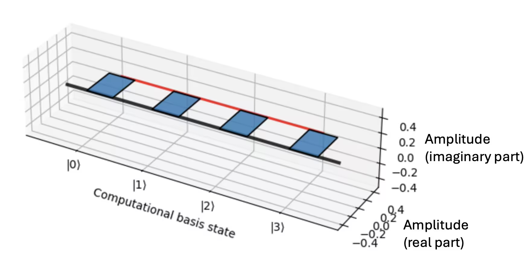
では、「フーリエ」基底状態はどのように理解すればよいのでしょうか？すべてのフーリエ基底状態は、すべての計算基底状態の等しい重ね合わせですが、各状態は構成要素の「位相」の周期性において異なります。これをより具体的に理解するために、2 Qubit システムの四つのフーリエ基底状態を見てみましょう。最も低次のフーリエ状態は、位相がまったく変化しないものです：

$|\phi_0\rangle = \frac{1}{2} (|00\rangle + |01\rangle + |10\rangle + |11\rangle)$

各項の複素振幅をプロットしてこの状態を可視化できます。赤い線は、計算基底状態の関数として複素平面上でこの振幅の位相がどのように回転するかを示すガイドです。$|\phi_0\rangle$ の場合、位相は一定のままです：

次のフーリエ基底状態は、構成要素の位相が $0$ から $2\pi$ まで一度だけ回転するものです：

$|\phi_1\rangle = \frac{1}{2} (|00\rangle + e^{i\pi/2}|01\rangle + e^{i\pi}|10\rangle + e^{3i\pi/2}|11\rangle) = \frac{1}{2}(|00\rangle + i|01\rangle - |10\rangle - i|11\rangle)$

複素振幅対計算基底状態のプロットでこの回転を確認できます：

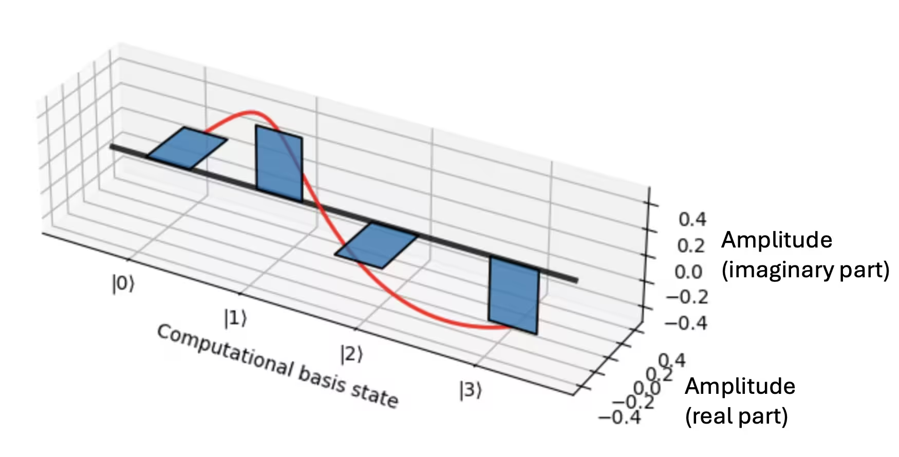
つまり、各状態の位相は、標準的な順序で並べたとき、一つ前の状態より $2\pi/4$ ラジアンずつ高くなっています。この例では基底状態が四つある（$N=4$）ためです。次の基底状態は $0$ から $2\pi$ まで二回転します：

$|\phi_2\rangle = \frac{1}{2} (|00\rangle + e^{i\pi}|01\rangle + e^{2i\pi}|10\rangle + e^{3i\pi}|11\rangle) = \frac{1}{2} (|00\rangle - |01\rangle + |10\rangle - |11\rangle)$

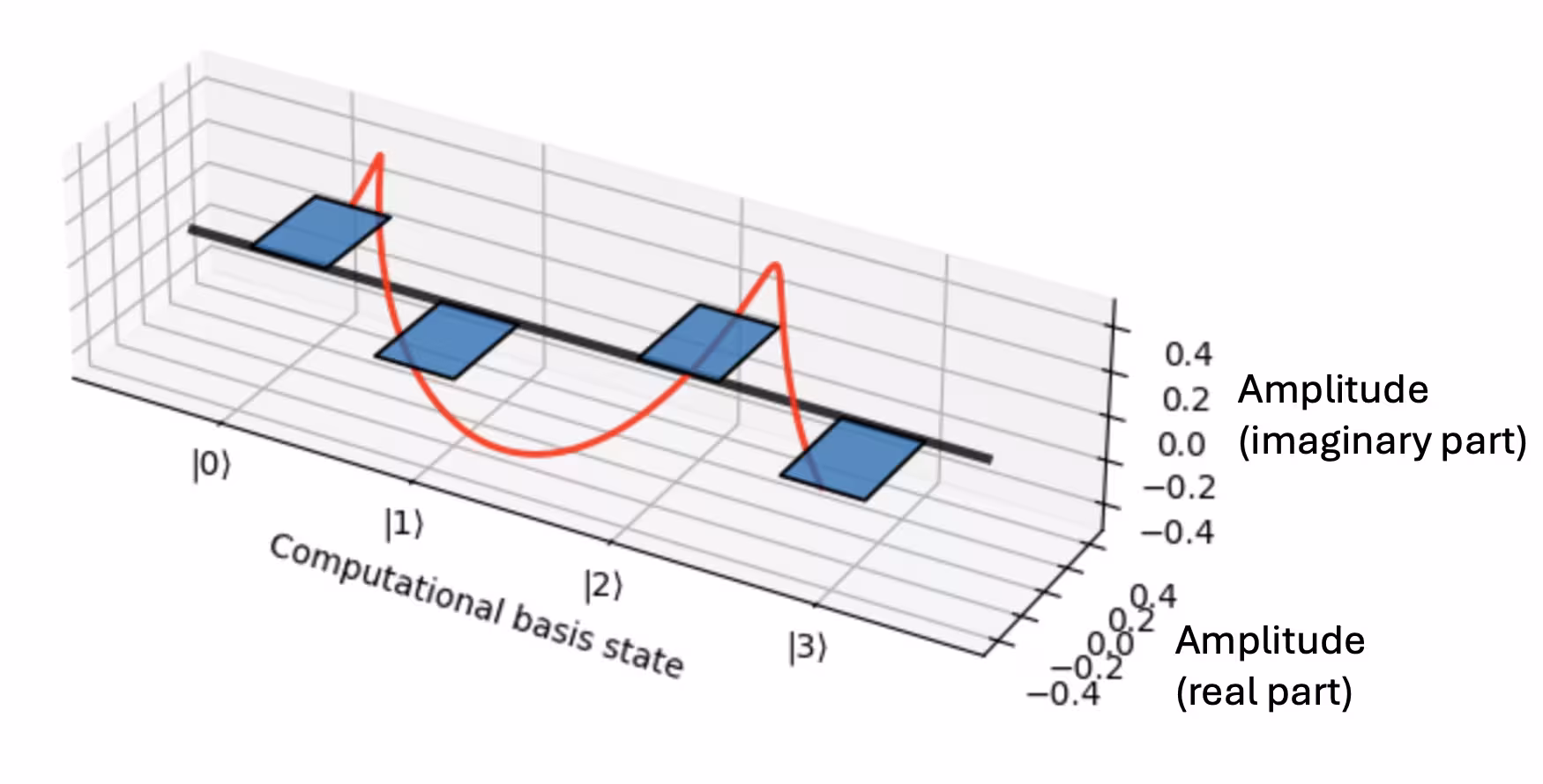
最後に、最も高次のフーリエ成分は位相の変化が最も速いものです。2 Qubit の例では、位相が $0$ から $2\pi$ まで三回転するものです：

$|\phi_3\rangle = \frac{1}{2} (|00\rangle + e^{3i\pi/2}|01\rangle + e^{6i\pi/2}|10\rangle + e^{9i\pi/2}|11\rangle) = \frac{1}{2} (|00\rangle - i|01\rangle - |10\rangle + i|11\rangle)$

一般に、$m$ Qubit の状態には $2^m$ 個のフーリエ基底状態があり、その位相変動の周波数は、$|\phi_0\rangle$ の場合の定数から $|\phi_{2^m-1}\rangle$ の場合の急速な変動まで幅があります。後者は重ね合わせ状態全体にわたって $2\pi$ を $2^m-1$ 回転します。したがって、量子状態に QFT を適用することは、冒頭で行った音楽波形の解析と基本的に同じ操作を行っていることになります。つまり、対象となる量子状態を構成するフーリエ周波数成分を特定しているのです。

QFT の例を試してみる

計算基底で状態を作成し、QFT を適用したときに何が起こるかを見ることで、量子フーリエ変換への直感をさらに養っていきましょう。ここでは、Qiskit Circuit Library の QFTGate を使って QFT をブラックボックスとして扱います。後ほど、その内部実装についても詳しく見ていきます。

まず、必要なパッケージを読み込み、Circuit を実行するデバイスを選択します：

import numpy as np
from qiskit import QuantumCircuit
from qiskit.visualization import plot_histogram
from qiskit.circuit.library import QFTGate

# Load the Qiskit Runtime service
from qiskit_ibm_runtime import QiskitRuntimeService

# Load the Runtime primitive and session
from qiskit_ibm_runtime import SamplerV2 as Sampler

service = QiskitRuntimeService()

# Use the least busy backend
# backend = service.least_busy(operational=True, simulator=False, min_num_qubits = 127)
backend = service.backend("ibm_pinguino2")

print(backend.name)

ibm_pinguino2

アカウントの利用可能時間がない場合や、何らかの理由でシミュレーターを使用したい場合は、以下のセルを実行することで、上で選択した量子デバイスを模倣するシミュレーターをセットアップできます：

# Load the backend sampler
from qiskit.primitives import BackendSamplerV2

# Load the Aer simulator and generate a noise model based on the currently-selected backend.
from qiskit_aer import AerSimulator
from qiskit_aer.noise import NoiseModel

noise_model = NoiseModel.from_backend(backend)

# Define a simulator using Aer, and use it in Sampler.
backend_sim = AerSimulator(noise_model=noise_model)
sampler_sim = BackendSamplerV2(backend=backend_sim)

# Alternatively, load a fake backend with generic properties and define a simulator.
from qiskit.providers.fake_provider import GenericBackendV2

backend_gen = GenericBackendV2(num_qubits=18)
sampler_gen = BackendSamplerV2(backend=backend_gen)

単一の計算基底状態

まず、単一の計算基底状態を変換してみましょう。ランダムな計算状態を作成することから始めます：

# Step 1: Map

qubits = 4
N = 2**qubits

qc = QuantumCircuit(qubits)

# flip state of random qubits to put in a random single computational basis state
for i in range(1, qubits):
    if np.random.randint(0, 2):
        qc.x(i)

# make a copy of the above circuit. (to be used when we apply the QFT in next part)
qc_qft = qc.copy()

qc.measure_all()
qc.draw("mpl")

# Step 2: Transpile
from qiskit.transpiler.preset_passmanagers import generate_preset_pass_manager

target = backend.target
pm = generate_preset_pass_manager(target=target, optimization_level=3)

qc_isa = pm.run(qc)

# Step 3: Run the job on a real quantum computer OR try fake backend

sampler = Sampler(mode=backend)
pubs = [qc_isa]

# Run the job on real quantum device

job = sampler.run(pubs, shots=1000)
res = job.result()
counts = res[0].data.meas.get_counts()

# OR Run the job on the Aer simulator with noise model from real backend

# job = sampler_sim.run([qc_isa])
# res = job.result()
# counts = res[0].data.meas.get_counts()

# Step 4: Post-Process
plot_histogram(counts)

では、QFTGate を使ってこの状態をフーリエ変換してみましょう：

# Step 1: Map

qc_qft.compose(QFTGate(qubits), inplace=True)
qc_qft.measure_all()
qc_qft.draw("mpl")

# Step 2: Transpile
from qiskit.transpiler.preset_passmanagers import generate_preset_pass_manager

target = backend.target
pm = generate_preset_pass_manager(target=target, optimization_level=3)

qc_isa = pm.run(qc_qft)

# Step 3: Run the job on a real quantum computer - try fake backend

sampler = Sampler(mode=backend)
pubs = [qc_isa]

# Run the job on real quantum device

job = sampler.run(pubs, shots=1000)
res = job.result()
counts = res[0].data.meas.get_counts()

# OR Run the job on the Aer simulator with noise model from real backend

# job = sampler_sim.run([qc_isa])
# res = job.result()
# counts = res[0].data.meas.get_counts()

# Step 4: Post-Process
plot_histogram(counts)

ご覧のとおり、実験的・統計的なノイズを多少考慮すると、各状態の占有確率はほぼ等しく測定されます。つまり、単一の計算基底状態に QFT を適用すると、結果はすべての状態の等しい重ね合わせになります。フーリエ変換に馴染みがあれば、これは驚くことではないでしょう。関数とそのフーリエ変換の間の直感的なつながりを構築する上で役立つ基本原理の一つは、「関数の幅とそのフーリエ変換の幅は逆比例する」というものです。したがって、時間領域で非常に局在した信号（たとえば極めて短いパルス）を生成するためには、広い範囲の周波数が必要です。その信号はフーリエ空間では非常に広くなります。

この事実は量子的な不確定性とも関係があります！ハイゼンベルクの不確定性原理は通常 $\Delta x \Delta p \ge \hbar / 2$ と表されます。位置の不確定性（$\Delta x$）が小さければ、運動量の不確定性（$\Delta p$）は大きくなければならず、その逆もまた然りです。位置基底 $x$ から運動量基底 $p$ への変換は、フーリエ変換によって実現されます。

注意：各基底状態における占有確率を測定しているため、重ね合わせの各部分間の相対的な位相に関する情報は失われることを念頭に置いてください。したがって、任意の単一の計算基底状態の QFT は、すべての基底状態にわたって同じ均等な占有確率の分布を示しますが、「位相」は必ずしも同じではありません。

二つの計算基底状態

次に、計算基底状態の重ね合わせを準備したらどうなるかを見てみましょう。この場合、フーリエ変換はどのようになると思いますか？

次の重ね合わせを選んでみましょう：

$|\psi\rangle = \frac{1}{\sqrt{2}} (|0\rangle + |N/2\rangle) = \frac{1}{\sqrt{2}} (|000...0\rangle + |100...0\rangle)$

# Step 1: Map
qubits = 4
N = 2**qubits

qc = QuantumCircuit(qubits)

# To make this state, we just need to apply a Hadamard to the last qubit

qc.h(qubits - 1)

qc_qft = qc.copy()

qc.measure_all()

qc.draw("mpl")

# First, let's go through steps 2-4 for the first circuit, qc

# Step 2: Transpile
from qiskit.transpiler.preset_passmanagers import generate_preset_pass_manager

target = backend.target
pm = generate_preset_pass_manager(target=target, optimization_level=3)

qc_isa = pm.run(qc)

# Step 3: Run the job on a real quantum computer - try fake backend

sampler = Sampler(mode=backend)
pubs = [qc_isa]

# Run the job on real quantum device

job = sampler.run(pubs, shots=1000)
res = job.result()
counts = res[0].data.meas.get_counts()

# OR run the job on the Aer simulator with noise model from real backend

# job = sampler_sim.run([qc_isa])
# res = job.result()
# counts = res[0].data.meas.get_counts()

# Step 4: Post-process
plot_histogram(counts)

では、QFTGate を使ってこの状態をフーリエ変換してみましょう：

# Step 1: Map

qc_qft.compose(QFTGate(qubits), inplace=True)
qc_qft.measure_all()
qc_qft.draw("mpl")

# Step 2: Transpile
from qiskit.transpiler.preset_passmanagers import generate_preset_pass_manager

target = backend.target
pm = generate_preset_pass_manager(target=target, optimization_level=3)

qc_isa = pm.run(qc_qft)

# Step 3: Run the job on a real quantum computer OR try fake backend

sampler = Sampler(mode=backend)
pubs = [qc_isa]

# Run the job on real quantum device

job = sampler.run(pubs, shots=1000)
res = job.result()
counts = res[0].data.meas.get_counts()

# OR run the job on the Aer simulator with noise model from real backend

# job = sampler_sim.run([qc_isa])
# res = job.result()
# counts = res[0].data.meas.get_counts()

# Step 4: Post-process
plot_histogram(counts)

これは少し驚くかもしれません。状態 $|\psi\rangle = \frac{1}{\sqrt{2}} (|0\rangle + |N/2\rangle)$ の QFT は、すべての偶数基底状態の重ね合わせのように見えます。しかし、各基底状態 $|\phi_y\rangle$ の可視化と、各成分の位相が $2\pi$ を $y$ 回転する様子を思い出すと、この結果が得られる理由が明らかになるかもしれません。

理解度チェック

以下の問いを読み、答えを考えてから、三角形をクリックして解答を確認してください。

上記のヒントを使って、$|\psi\rangle = \frac{1}{\sqrt{2}} (|0\rangle + |N/2\rangle)$ の QFT として得られた結果がなぜ予想どおりなのかを説明してください。

解答：

元の状態は、重ね合わせの2つの部分の間に相対位相が 0（または $2\pi$ の整数倍）を持っています。したがって、この状態は、そのような形で位相が一致するフーリエ成分を持つことがわかります。すなわち、|0000> の項と |1000> の項の間の位相シフトが 0 となるものです。各フーリエ基底状態 $|\phi_y\rangle$ は、位相が $2\pi y/N$ の速度で累積する項で構成されています。これは、通常の順序で並べたとき、重ね合わせの各項が直前の項より $2\pi y/N$ だけ大きい位相を持つことを意味します。したがって、中間点 $N/2$ において、位相 $2\pi y/N \times N/2$ が $2\pi$ の整数倍になることが求められます。これは $y$ が偶数のときに成り立ちます。

すべての奇数の二進数にピークを持つ QFT に対応する計算基底状態の重ね合わせはどのようなものでしょうか？

解答：

状態 $\psi = |0\rangle - |N/2\rangle$ の QFT を計算すると、すべての奇数の二進数の状態にピークが現れます。

QFT アルゴリズムを詳しく見る

計算基底とフーリエ基底における Qubit 状態の関係についての直観が深まったところで、QFT アルゴリズム自体を詳しく見ていきましょう。つまり、この変換を実現するために量子コンピューターに実際にどのような Gate を適用するのでしょうか？

まず、1つの Qubit という小さなケースから始めましょう。そのため、基底状態は2つです。QFT$_2$ は計算基底状態 $|0\rangle$ と $|1\rangle$ をフーリエ基底状態 $\phi_0$ と $\phi_1$ へと変換します。

$|\phi_0\rangle = \frac{1}{\sqrt{2}}(|0\rangle + |1\rangle)$

$|\phi_1\rangle = \frac{1}{\sqrt{2}}(|0\rangle - |1\rangle)$

理解度チェック

以下の問いを読み、答えを考えてから、三角形をクリックして解答を確認してください。

前のセクションの QFT の式を使って、上記の2つのフーリエ基底状態を検証してください。

解答：

一般的な QFT の式は次のとおりです。

$| \phi_y \rangle = \frac{1}{\sqrt{N}}\sum_{x=0}^{N-1}\omega_N^{y x} \vert x \rangle$

1つの Qubit（$n=1$）の場合、$N=2^n=2$ であり、$\omega_N^{xy} = e^{2\pi i \frac {y x}{2}}$ です。したがって、

$| \phi_0 \rangle = \frac{1}{\sqrt{2}}(e^{2\pi i \frac {0 \times 0}{2}}|0\rangle + e^{2\pi i \frac {0 \times 1}{2}}|1\rangle) = \frac{1}{\sqrt{2}}(|0\rangle + |1\rangle)$

$| \phi_1 \rangle = \frac{1}{\sqrt{2}}(e^{2\pi i \frac {1 \times 0}{2}}|0\rangle + e^{2\pi i \frac {1 \times 1}{2}}|1\rangle) = \frac{1}{\sqrt{2}}(|0\rangle - |1\rangle)$

これら2つの式をよく見てください。この変換を実装するために使える量子 Gate をすでに知っているかもしれません。つまり、計算基底状態 $|0\rangle$ と $|1\rangle$ をそれぞれのフーリエ基底状態 $|\phi_0\rangle$ と $|\phi_1\rangle$ に変換する Gate が存在します。それはアダマール Gate です！ QFT$_N$ 演算の行列表現を導入すると、これはさらに明確になります。

$\text{QFT}_N = \frac{1}{\sqrt{N}} \sum_{x=0}^{N-1} \sum_{y=0}^{N-1} \omega_N^{xy} \vert x \rangle \langle y \vert$

この表記法で量子演算子を表す方法に慣れていなくても、問題ありません！ これは $N \times N$ 行列を表す方法で、$x$ と $y$ が $0$ から $N-1$ までの行列の列と行のインデックスを示し、$\omega_N^{xy}$ がその特定の要素の値です。たとえば、第 0 列・第 2 行の要素は単に $\omega_N^{0,2} = e^{2 \pi i \frac{0 \times 2}{N}} = 1$ となります。

この表現では、各計算基底状態は基底ベクトルの一つに対応します。

$$\begin{pmatrix} 1 \\ 0 \\ \vdots \\ 0 \end{pmatrix}, |1\rangle = \begin{pmatrix} 0 \\ 1 \\ \vdots \\ 0 \end{pmatrix}, |N-1\rangle = \begin{pmatrix} 0 \\ 0 \\ \vdots \\ 1 \end{pmatrix}.$$

この表現についてより深く学びたい場合は、量子情報の基礎コースにある複数システムに関する John Watrous のレッスンを参照してください。

QFT$_4$ の行列を構成してみましょう。上の式を使うと、

\text\{QFT\}_4 = \frac\{1\}\{2\} \begin\{pmatrix\} 1 & 1 & 1 & 1 \\ 1 & i & -1 & -i \\ 1 & -1 & 1 & -1 \\ 1 & -i & -1 & i \\ \end\{pmatrix\}

この行列を量子コンピューターで実装するには、どの Qubit にどの Gate を組み合わせて適用すれば上記の行列に一致するユニタリー変換が得られるかを考える必要があります。必要な Gate の一つはすでにわかっています：アダマールです。もう一つ必要な Gate は制御位相 Gate です。これは、制御 Qubit が状態 $|1\rangle$ にある場合に限り、ターゲット Qubit の状態に相対位相 $\alpha$ を適用します。行列形式では次のようになります。

\text\{CP\}_\alpha = \begin\{pmatrix\} 1 & 0 & 0 & 0 \\ 0 & 1 & 0 & 0 \\ 0 & 0 & 1 & 0 \\ 0 & 0 & 0 & e^\{i\alpha\} \\ \end\{pmatrix\}

変化するのは状態 $|11\rangle$ のみであるため、どちらの Qubit を「制御」とし、どちらを「ターゲット」と見なしても実際には問題ありません。結果はどちらも同じになります。

最後に、SWAP Gate もいくつか必要です。SWAP Gate は2つの Qubit の状態を交換します。その形は次のとおりです。

\text\{SWAP\}_\alpha = \begin\{pmatrix\} 1 & 0 & 0 & 0 \\ 0 & 0 & 1 & 0 \\ 0 & 1 & 0 & 0 \\ 0 & 0 & 0 & 1 \\ \end\{pmatrix\}

$m$ Qubit 上に QFT$_{2^m}$ Circuit を構成する手順は反復的です。まず Qubit $1$ から $m-1$ に QFT$_{2^{m-1}}$ を適用し、次に Qubit $0$ と他の $m-1$ Qubit の間にいくつかの Gate を追加します。しかし QFT$_{2^{m-1}}$ を適用するには、まず Qubit $2$ から $m-1$ に QFT$_{2^{m-2}}$ を適用し、次に Qubit $1$ と残りの Qubit $2$ から $m-1$ の間に Gate を追加する必要があります。これはロシアの入れ子人形のようなものです：各人形は QFT Circuit の次元を2倍にし、最も小さな人形が中心に位置する QFT$_2$、すなわちアダマール Gate です。

次のサイズの人形の中に人形を入れる（つまり QFT の次元を2倍にする）には、常に同じ手順に従います。

1. まず、下位 $m-1$ Qubit に QFT$_{2^{m-1}}$ を適用します。これが、次のサイズの人形の中に入れるロシアの入れ子人形セットの「小さな人形」です。
2. その1つ上の Qubit を制御として使用し、残りの $m-1$ Qubit それぞれの標準基底状態に対応する位相で、下位 $m-1$ Qubit 各々に制御位相 Gate を適用します。
3. 位相 Gate の制御に使用したのと同じ最上位 Qubit にアダマールを実行します。
4. SWAP Gate を使って Qubit の順序を並べ替え、最下位（先頭）ビットが最上位（末尾）ビットになり、他のすべてが1つ上にシフトするようにします。

これまで Qiskit の Circuit ライブラリの QFTGate 関数を使用してきましたが、ここで上記の手順を検証するために、これらの QFT Gate の内部を decompose() で確認してみましょう。

qc = QuantumCircuit(1)
qc.compose(QFTGate(1), inplace=True)
qc.decompose().draw("mpl")

qc = QuantumCircuit(2)
qc.compose(QFTGate(2), inplace=True)
qc.decompose().draw("mpl")

qc = QuantumCircuit(3)
qc.compose(QFTGate(3), inplace=True)
qc.decompose().draw("mpl")

qc = QuantumCircuit(4)
qc.compose(QFTGate(4), inplace=True)
qc.decompose().draw("mpl")

最初の4つの QFT を見ることで、それぞれが次に大きなものの中に入れ子になっている様子が見えてくるはずです。ただし、いくつかの位相 Gate が上で概説した手順とは厳密に異なっており、SWAP が各サブルーティンの後ではなく、完全な QFT の最後にのみ現れることに気づいたかもしれません。これは不要な Gate を省くためで、それによって Circuit の実行時間を短縮し、エラーを減らすことができます。入れ子の人形ごとに SWAP を実装する代わりに、Circuit は各 Qubit 状態があるべき位置を追跡し、それに応じて位相 Gate を適用する Qubit を調整します。そして最後に、最終的な SWAP のセットですべてを適切な位置に配置します。

QFT の応用：位相推定

QFT が量子コンピューティングにおける有用な問題を解決するためにどのように使えるかを見ていきましょう。逆量子フーリエ変換の計算は、量子位相推定（QPE）と呼ばれるアルゴリズムに必要なステップであり、QPE 自体もショアの素因数分解アルゴリズムを含む多くのアルゴリズムのサブルーティンとして使われています。

QPE の目標は、ユニタリー演算子の固有値を推定することです。ユニタリー演算子は量子コンピューティングで至るところに登場し、その関連する固有ベクトルの固有値を求めることは、より大きなアルゴリズムの必要なステップであることがよくあります。問題によって、固有値はシミュレーション型の問題におけるハミルトニアンのエネルギーを表したり、ショアのアルゴリズムで数の素因数を見つける助けになったり、その他の重要な情報を含んだりします。QPE は量子コンピューティングで最も重要かつ広く使われているサブルーティンの一つです。

では、これが量子フーリエ変換とどのような関係があるのでしょうか？ 思い出していただけるように、ユニタリー演算子の固有値 $\lambda$ は大きさ $|\lambda| = 1$ を持ちます。そのため、各固有値を大きさ1の複素数として書くことができます。

$\lambda = e^{2\pi i \theta}$

ここで $\theta$ は 0 と 1 の間の実数です。ユニタリー行列の詳細については、量子情報の基礎における John Watrous の関連レッスンを参照してください。

$\lambda$ は $\theta$ に関して周期的であることに注目してください。QFT が周期的な関数の分析にいかに有用かを見てきたことから、すでに QFT が関係しているのではないかと思われたかもしれません。以下では、アルゴリズムを順を追って説明し、QFT がどのように登場するかを正確に見ていきます。

QPE の仕組み

まず、最もシンプルな QPE アルゴリズムから始めます。このアルゴリズムは位相を1ビットの精度で大まかに推定します。言い換えれば、$\theta = 0$ と $\theta = 1/2$ を区別できますが、それ以上の精度は持ちません。以下が Circuit 図です。

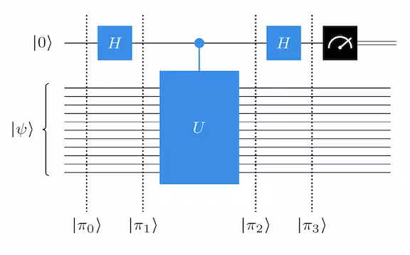
Qubit は状態 $|\pi_0\rangle = |\psi\rangle|0\rangle$ に準備されます。ここで Qubit $0$ は状態 $|0\rangle$ にあり、残りの Qubit は $U$ の固有状態 $|\psi\rangle$ にあります。最初のアダマールの後、Qubit の状態は次のようになります。

$|\pi_1\rangle = \frac{1}{\sqrt{2}}|\psi\rangle (|0\rangle + |1\rangle)$

次の Gate は「制御-$U$」Gate です。これは、Qubit $0$ が状態 $|1\rangle$ にある場合に状態 $|\psi\rangle$ にある下位 Qubit にユニタリー演算 $U$ を適用し、Qubit $0$ が状態 $|0\rangle$ にある場合は $|\psi\rangle$ に何もしません。これにより Qubit は次の状態に変換されます。

$|\pi_2\rangle = \frac{1}{\sqrt{2}}( |\psi\rangle|0\rangle + e^{2\pi i \theta}|\psi\rangle|1\rangle)$ $= \frac{1}{\sqrt{2}}|\psi\rangle (|0\rangle + e^{2\pi i \theta}|1\rangle)$

ここで不思議なことが起きました。制御-$U$ Gate は Qubit $0$ のみを制御 Qubit として使うため、この Gate が Qubit $0$ の状態を変えないと思うかもしれません。しかし実際には変わります！ 演算が下位 Qubit に適用されたにもかかわらず、Gate の全体的な効果は Qubit $0$ の位相を変えることです。これは「位相キックバック機構」として知られており、ドイチュ・ジョザやグローバーのアルゴリズムを含む多くの量子アルゴリズムで使用されています。位相キックバック機構の詳細については、量子アルゴリズムの基礎における量子クエリアルゴリズムに関する John Watrous のレッスンを参照してください。

位相キックバックの後、Qubit $0$ にもう一つアダマールを適用すると、次の状態になります。

$|\pi_3\rangle = |\psi\rangle ( \frac{1+e^{2\pi i \theta}}{2} |0\rangle + \frac{1 - e^{2\pi i \theta}}{2}|1\rangle) = |\psi\rangle ( \cos(\pi\theta) |0\rangle - i \sin(\pi\theta)|1\rangle)$

したがって、最後に Qubit $0$ を測定すると、$\theta = 0$ の場合は 100% の確率で $|0\rangle$ が測定され、$\theta = \frac{1}{2}$ の場合は 100% の確率で $|1\rangle$ が測定されます（量子コンピューターが完全でノイズがない場合）。$\theta$ がこれ以外の値の場合、最終的な測定は確率的になり、限られた情報しか得られません。

より高精度の QPE：より多くの Qubit

このシンプルな概念を任意の精度を持つより複雑なアルゴリズムに拡張できます。位相を測定するために Qubit $0$ だけを使う代わりに、$m$ 個の Qubit $0$ から $m-1$ を使うことで、$m$ ビットの精度で位相を推定できるようになります。これがどのように機能するか見てみましょう。

この高精度 QPE Circuit は1ビット版と同じように始まります。最初の $m$ 個の Qubit にアダマールが適用され、残りの Qubit は状態 $|\psi\rangle$ に準備され、次の状態が作られます。

$|\pi_1\rangle = \frac{1}{2^{m/2}}|\psi\rangle(|0\rangle+|1\rangle)(|0\rangle+|1\rangle)...(|0\rangle+|1\rangle)$

次に、制御ユニタリーが適用されます。Qubit $0$ は以前と同じユニタリー $U$ の制御です。しかし今度は、Qubit $1$ がユニタリー $U^2$（単純に $U$ を2回適用したもの）の制御になります。よって $U^2$ の固有値は $e^{2*2\pi i \theta}$ です。一般的に、$0$ から $m-1$ までの各 Qubit $k$ はユニタリー $U^{2^k}$ の制御になります。これは、これらの Qubit それぞれが $e^{2^k*2\pi i \theta}$ の位相キックバックを受けることを意味します。その結果、次の状態になります。

$|\pi_2\rangle = |\psi\rangle \otimes \frac{1}{2^{m/2}} (|0\rangle+e^{2^{m-1}2\pi i \theta}|1\rangle)(|0\rangle+e^{2^{m-2}2\pi i \theta}|1\rangle)...(|0\rangle+e^{2\pi i \theta}|1\rangle)$

これは計算基底状態の和として書き直すことができます。

$|\pi_2\rangle = |\psi\rangle \otimes \frac{1}{2^{m/2}} \sum_{k=0}^{2^{m}-1} e^{2\pi i k \theta} |k\rangle$

この和に見覚えはありませんか？ これは QFT です！ 量子フーリエ変換の式を思い出してください。

$\text{QFT}_{2^m}| y \rangle = \frac{1}{\sqrt{2^m}}\sum_{x=0}^{2^m-1}\omega_{2^m}^{y x} \vert x \rangle$

したがって、位相 $\theta = y/2^m$ が $0$ から $2^m-1$ の間の整数 $y$ に対して成り立つ場合、この状態に逆 QFT を適用すると次の状態が得られます。

$|\pi_3\rangle = |\psi\rangle \otimes |y\rangle$

そして $|y\rangle$ から $\theta$ を求めることができます。

一方、$\theta/2^m$ が整数倍でない場合、逆 QFT を適用しても $\theta$ を近似することしかできません。どれだけ近似できるかは確率的であり、常に最良の近似が得られるわけではありませんが、かなり近い値が得られます。また、使用する Qubit 数 $m$ が多いほど、より良い近似が得られます。$\theta$ のこの近似をどのように定量化するかについては、量子アルゴリズムの基礎における位相推定と素因数分解に関する John Watrous のレッスンをご確認ください。

まとめ

このモジュールでは、QFT とは何か、量子コンピューターでどのように実装するか、そして問題解決においていかに有用かの概要を説明しました。量子位相推定で固有値について学ぶためにどのように使えるかを見たことで、その有用性の一端に触れていただけたと思います。

重要な概念

• 量子フーリエ変換は離散フーリエ変換の量子版です。
• QFT は基底変換の例です。
• 量子位相推定の手順は、制御ユニタリー演算による位相キックバック機構と逆 QFT に依存しています。
• QFT と QPE はどちらも数多くの量子アルゴリズムで広く使われているサブルーティンです。

問題

正誤問題

1. 正誤：量子フーリエ変換は古典的な離散フーリエ変換（DFT）の量子版である。
2. 正誤：QFT はアダマール Gate と CNOT Gate のみを使って実装できる。
3. 正誤：QFT はショアのアルゴリズムの重要な構成要素である。
4. 正誤：量子位相推定の出力は、演算子の固有ベクトルを表す量子状態である。
5. 正誤：QPE では逆量子フーリエ変換（QFT$^\dag$）の使用が必要である。
6. 正誤：QPE において、位相 $\phi$ が $n$ ビットで正確に表現できる場合、アルゴリズムは確率1で正確な結果を与える。

短答問題

1. $2^n$ 個のデータ点を持つシステムに対して QFT を実行するには、何個の Qubit が必要ですか？
2. QFT は計算基底状態でない状態に対して使用できますか？ 可能な場合、どのようになりますか？
3. QPE で使用する制御 Qubit の数は、得られる位相推定の分解能にどのように影響しますか？

問題

1. 行列の掛け算を使って、QFT アルゴリズムの各ステップが確かに $\text{QFT}_4$ 行列になることを検証してください。

$$\text{QFT}_4 = \frac{1}{2} \begin{pmatrix} 1 & 1 & 1 & 1 \\ 1 & i & -1 & -i \\ 1 & -1 & 1 & -1 \\ 1 & -i & -1 & i \\ \end{pmatrix}$$

（手計算をする必要はありません！）

チャレンジ問題

1. すべての奇数の計算基底の等しい重ね合わせである4 Qubit の状態 $|\psi\rangle = |0001\rangle + |0011\rangle + |0101\rangle + |0111\rangle +|1001\rangle +|1011\rangle +|1101\rangle +|1111\rangle$ を作ってください。次に、その状態に対して QFT を実行してください。得られた状態はどのようなものですか？ フーリエ変換の知識を使って、結果がなぜそのようになるかを説明してください。