量子変分回路と量子ニューラルネットワーク

このレッスンでは、データ分類タスクに向けていくつかの変分量子回路を実装します。これらは変分量子分類器（VQC）と呼ばれます。かつては、古典的なニューラルネットワークとの類比から、VQCの一部を量子ニューラルネットワーク（QNN）と呼ぶことが一般的でした。実際、畳み込み層のような古典ニューラルネットワークから借用された構造がVQCで重要な役割を果たす場合があります。類比が強い場合には、QNNという呼び方が有用かもしれません。しかし、パラメータ化された量子回路は必ずしもニューラルネットワークの一般的な構造に従う必要はありません。例えば、すべてのデータを最初の（入力）層に読み込む必要はなく、最初の層にデータの一部を読み込み、いくつかのゲートを適用した後、追加のデータを読み込む（データの「再アップロード」と呼ばれるプロセス）ことができます。したがって、QNNはパラメータ化された量子回路のサブセットと考えるべきであり、古典ニューラルネットワークとの類比によって有用な量子回路の探索が制限されるべきではありません。

このレッスンで扱うデータセットは、水平線と垂直線を含む画像から成り立っており、目標は未見の画像を線の向きに応じて2つのカテゴリのいずれかにラベル付けすることです。これをVQCで実現します。進めながら、計算を改善・スケールアップする方法についても説明します。ここで使用するデータセットは古典的に非常に簡単に分類できます。このデータセットはシンプルさを重視して選ばれており、この問題の量子的な部分に集中し、データセットの属性が量子回路のどの部分に対応するかを確認できるようにしています。古典アルゴリズムがこれほど効率的な単純なケースでは、量子速度向上を期待することは合理的ではありません。

このレッスンの終わりまでに、以下のことができるようになります：

画像から量子回路にデータを読み込む
VQC（またはQNN）のアンザッツを構築し、問題に合わせて調整する
VQC/QNNを訓練し、テストデータに対して正確な予測を行う
問題をスケールアップし、現在の量子コンピューターの限界を認識する

データ生成

まずデータを構築します。データセットはQiskitパターンフレームワークの一部として明示的に生成されることは少ないですが、データの種類と前処理は量子コンピューティングを機械学習に正しく適用するために重要です。以下のコードは、固定ピクセル寸法の画像データセットを定義します。画像の1行または1列全体に値 $\pi/2$ が割り当てられ、残りのピクセルには区間 $(0,\pi/4)$ 上のランダムな値が割り当てられます。ランダムな値はデータのノイズです。画像がどのように生成されるかを理解するためにコードを一読してください。後ほど画像のスケールを拡大します。

# Added by doQumentation — required packages for this notebook
!pip install -q matplotlib numpy qiskit qiskit-ibm-runtime scipy scikit-learn

# This code defines the images to be classified:

import numpy as np

# Total number of "pixels"/qubits
size = 8
# One dimension of the image (called vertical, but it doesn't matter). Must be a divisor of `size`
vert_size = 2
# The length of the line to be detected (yellow). Must be less than or equal to the smallest dimension of the image (`<=min(vert_size,size/vert_size)`
line_size = 2

def generate_dataset(num_images):
    images = []
    labels = []
    hor_array = np.zeros((size - (line_size - 1) * vert_size, size))
    ver_array = np.zeros((round(size / vert_size) * (vert_size - line_size + 1), size))

    j = 0
    for i in range(0, size - 1):
        if i % (size / vert_size) <= (size / vert_size) - line_size:
            for p in range(0, line_size):
                hor_array[j][i + p] = np.pi / 2
            j += 1

    # Make two adjacent entries pi/2, then move down to the next row. Careful to avoid the "pixels" at size/vert_size - linesize, because we want to fold this list into a grid.

    j = 0
    for i in range(0, round(size / vert_size) * (vert_size - line_size + 1)):
        for p in range(0, line_size):
            ver_array[j][i + p * round(size / vert_size)] = np.pi / 2
        j += 1

    # Make entries pi/2, spaced by the length/rows, so that when folded, the entries appear on top of each other.

    for n in range(num_images):
        rng = np.random.randint(0, 2)
        if rng == 0:
            labels.append(-1)
            random_image = np.random.randint(0, len(hor_array))
            images.append(np.array(hor_array[random_image]))

        elif rng == 1:
            labels.append(1)
            random_image = np.random.randint(0, len(ver_array))
            images.append(np.array(ver_array[random_image]))
            # Randomly select 0 or 1 for a horizontal or vertical array, assign the corresponding label.

        # Create noise
        for i in range(size):
            if images[-1][i] == 0:
                images[-1][i] = np.random.rand() * np.pi / 4
    return images, labels

hor_size = round(size / vert_size)

上記のコードでは、画像が垂直線（+1）または水平線（-1）を含むかどうかを示すラベルも生成されています。次に、sklearnを使用して100枚の画像からなるデータセットをトレーニング用とテスト用に分割します（対応するラベルも含む）。ここでは、データセットの $70\%$ をトレーニングに使用し、残りの $30\%$ をテスト用に保留します。

from sklearn.model_selection import train_test_split

np.random.seed(42)
images, labels = generate_dataset(200)

train_images, test_images, train_labels, test_labels = train_test_split(
    images, labels, test_size=0.3, random_state=246
)

データセットのいくつかの要素をプロットして、これらの線がどのように見えるかを確認しましょう：

import matplotlib.pyplot as plt

# Make subplot titles so we can identify categories
titles = []
for i in range(8):
    title = "category: " + str(train_labels[i])
    titles.append(title)

# Generate a figure with nested images using subplots.
fig, ax = plt.subplots(4, 2, figsize=(10, 6), subplot_kw={"xticks": [], "yticks": []})

for i in range(8):
    ax[i // 2, i % 2].imshow(
        train_images[i].reshape(vert_size, hor_size),
        aspect="equal",
    )
    ax[i // 2, i % 2].set_title(titles[i])
plt.subplots_adjust(wspace=0.1, hspace=0.3)

前のコードセルの出力

これらの画像はそれぞれ、シンプルなリスト形式で train_labels 内のラベルと対応しています：

print(train_labels[:8])

[1, 1, 1, 1, -1, 1, 1, 1]

変分量子分類器：最初の試み

Qiskitパターンのステップ1：問題を量子回路にマッピングする

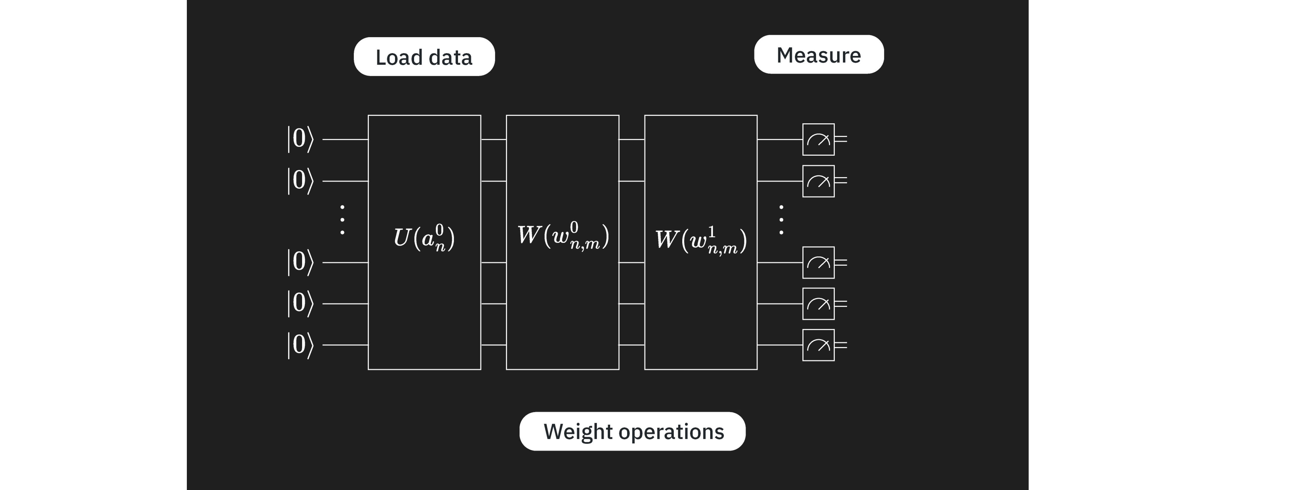
目標は、データベクトル／画像 $\vec{x}$ を正しいカテゴリにマッピングする、パラメータ $\theta$ を持つ関数 $f$ を見つけることです： $f_\theta(\vec{x}) \rightarrow \pm1$ 。これは少数の層を持つVQCを使って実現します。各層はそれぞれ異なる役割を持ちます：

f_\theta(\vec{x}) = \langle 0|U^{\dagger}(\vec{x})W^\dagger(\theta)OW(\theta)U(\vec{x})|0\rangle

ここで、 $U(\vec{x})$ はエンコーディング回路であり、前のレッスンで見たように多くの選択肢があります。 $W(\theta)$ は変分（訓練可能な）回路ブロックであり、 $\theta$ は訓練されるパラメータのセットです。これらのパラメータは、古典的な最適化アルゴリズムによって変化させ、量子回路による画像の最良の分類をもたらすパラメータセットを見つけます。この変分回路は「アンザッツ」と呼ばれることもあります。最後に、 $O$ はEstimatorプリミティブを使って推定されるオブザーバブルです。層をこの順番に配置したり、完全に分離したりする制約はありません。技術的な動機に基づく任意の順序で複数の変分層やエンコーディング層を持つことができます。

まず、データをエンコードするための特徴マップを選択します。他のいくつかの特徴マッピングと比較して回路深度を低く保つことができる z_feature_map を使用します。

from qiskit.circuit.library import z_feature_map

# One qubit per data feature
num_qubits = len(train_images[0])

# Data encoding
# Note that qiskit orders parameters alphabetically. We assign the parameter prefix "a" to ensure our data encoding goes to the first part of the circuit, the feature mapping.
feature_map = z_feature_map(num_qubits, parameter_prefix="a")

次に、訓練するアンザッツを決定する必要があります。アンザッツを選択する際にはさまざまな考慮事項があります。完全な説明はこの入門の範囲を超えますが、ここではいくつかのカテゴリの考慮事項を簡単に示します。

ハードウェア： 現代の量子コンピューターはすべて、古典的な対応物よりもエラーが発生しやすく、ノイズの影響を受けやすいです。過度に深いアンザッツ（特にトランスパイルされた2量子ビット深度）を使用しても良い結果は得られません。関連する問題として、量子コンピューターには何らかの量子ビットレイアウトがあり、一部の物理量子ビットは量子コンピューター上で隣接しており、他のものは非常に離れている場合があります。隣接する量子ビットをエンタングルしても深度はあまり増加しませんが、非常に離れた量子ビットをエンタングルすると、隣接する量子ビット上に情報を移動させるためにスワップゲートを挿入する必要があるため、深度が大幅に増加する可能性があります。
問題： アンザッツを導くような問題に関する情報がある場合は、それを活用してください。例えば、このレッスンのデータは水平線と垂直線の画像で構成されています。隣接する色／値のどのような相関が水平または垂直線の画像を識別するかを考えてみましょう。隣接するピクセルに対応するクビット間のこの相関にはアンザッツのどのような属性が対応するでしょうか？この点については後ほどより技術的に再検討します。しかし今は、隣接するピクセルに対応する量子ビット間にエンタングルメントとCNOTゲートを含めることが良いアイデアのように思えると言うに留めましょう。より広い視野では、問題が実際に量子回路を使って最もよく解かれるかどうか、あるいは同様の仕事ができる古典アルゴリズムが存在するかどうかを検討してください。
パラメータ数： 回路内の独立にパラメータ化された各量子ゲートは古典的に最適化される空間を増加させ、収束が遅くなります。しかし問題がスケールアップするにつれて、バレンプラトーに遭遇する可能性があります。この用語は、問題サイズが増加するにつれて変分量子アルゴリズムの最適化ランドスケープが指数関数的に平坦でフィーチャーレスになる現象を指します。これにより勾配が消失し、アルゴリズムを効果的に訓練することが困難になります[1]。バレンプラトーはVQC/QNNのような変分量子アルゴリズムに関連します。パラメータ数の増加がバレンプラトーを回避するための唯一の考慮事項ではないことに注意してください。他の考慮事項にはグローバルコスト関数やランダムパラメータ初期化などが含まれます。

このレッスンでは、アンザッツ構築における良い実践のいくつかの簡単な例を見ていきます。まず以下のアンザッツを試しましょう。後ほど改訂します。

# Import the necessary packages
from qiskit import QuantumCircuit
from qiskit.circuit import ParameterVector

# Initialize the circuit using the same number of qubits as the image has pixels
qnn_circuit = QuantumCircuit(size)

# We choose to have two variational parameters for each qubit.
params = ParameterVector("θ", length=2 * size)

# A first variational layer:
for i in range(size):
    qnn_circuit.ry(params[i], i)

# Here is a list of qubit pairs between which we want CNOT gates. The choice of these is not yet obvious.
qnn_cnot_list = [[0, 1], [1, 2], [2, 3]]

for i in range(len(qnn_cnot_list)):
    qnn_circuit.cx(qnn_cnot_list[i][0], qnn_cnot_list[i][1])

# The second variational layer:
for i in range(size):
    qnn_circuit.rx(params[size + i], i)

# Check the circuit depth, and the two-qubit gate depth
print(qnn_circuit.decompose().depth())
print(
    f"2+ qubit depth: {qnn_circuit.decompose().depth(lambda instr: len(instr.qubits) > 1)}"
)

# Draw the circuit
qnn_circuit.draw("mpl")

5
2+ qubit depth: 3

┌──────────┐             ┌──────────┐
q_0: ┤ Ry(θ[0]) ├──────■──────┤ Rx(θ[8]) ├─────────────────────────
     ├──────────┤    ┌─┴─┐    └──────────┘┌──────────┐
q_1: ┤ Ry(θ[1]) ├────┤ X ├─────────■──────┤ Rx(θ[9]) ├─────────────
     ├──────────┤    └───┘       ┌─┴─┐    └──────────┘┌───────────┐
q_2: ┤ Ry(θ[2]) ├────────────────┤ X ├─────────■──────┤ Rx(θ[10]) ├
     ├──────────┤                └───┘       ┌─┴─┐    ├───────────┤
q_3: ┤ Ry(θ[3]) ├────────────────────────────┤ X ├────┤ Rx(θ[11]) ├
     ├──────────┤┌───────────┐               └───┘    └───────────┘
q_4: ┤ Ry(θ[4]) ├┤ Rx(θ[12]) ├─────────────────────────────────────
     ├──────────┤├───────────┤
q_5: ┤ Ry(θ[5]) ├┤ Rx(θ[13]) ├─────────────────────────────────────
     ├──────────┤├───────────┤
q_6: ┤ Ry(θ[6]) ├┤ Rx(θ[14]) ├─────────────────────────────────────
     ├──────────┤├───────────┤
q_7: ┤ Ry(θ[7]) ├┤ Rx(θ[15]) ├─────────────────────────────────────
     └──────────┘└───────────┘

データエンコーディングと変分回路が準備できたので、それらを組み合わせて完全なアンザッツを形成します。この場合、量子回路のコンポーネントはニューラルネットワークのものと非常に類似しており、 $U(\vec{x})$ は画像から入力値を読み込む層に最も似ており、 $W(\theta)$ は可変「重み」の層に似ています。この類比がこの場合に成立するため、命名規則の一部に「qnn」を採用しています。しかし、この類比はVQCの探索において制限的であるべきではありません。

# QNN ansatz
ansatz = qnn_circuit

# Combine the feature map with the ansatz
full_circuit = QuantumCircuit(num_qubits)
full_circuit.compose(feature_map, range(num_qubits), inplace=True)
full_circuit.compose(ansatz, range(num_qubits), inplace=True)

# Display the circuit
full_circuit.decompose().draw("mpl", style="clifford", fold=-1)

前のコードセルの出力

オブザーバブルを定義する必要があります。コスト関数で使用するためです。Estimatorを使用してこのオブザーバブルの期待値を取得します。問題に動機づけられた良いアンザッツを選択していれば、各量子ビットには分類に関連する情報が含まれます。情報をより少ない量子ビットに統合するための層（畳み込み層と呼ばれる）を追加して、回路内の量子ビットのサブセットのみで測定が必要になるようにすることができます（畳み込みニューラルネットワークのように）。または、各量子ビットから何らかの属性を測定することもできます。ここでは後者を選択するので、各量子ビットに Z 演算子を含めます。 $Z$ を選択することに特別な制約はありませんが、よく動機づけられています：

これは二値分類タスクであり、 $Z$ の測定は2つの可能な結果を生じさせます。
$Z$ の固有値（ $\pm 1$ ）は適度に分離されており、区間 [-1, +1] 内のEstimator結果をもたらします。0 は単純にカットオフ値として使用できます。
Pauli Z 基底で測定するのは余分なゲートオーバーヘッドなしで簡単です。

したがって、Z は非常に自然な選択です。

from qiskit.quantum_info import SparsePauliOp

observable = SparsePauliOp.from_list([("Z" * (num_qubits), 1)])

量子回路と推定したいオブザーバブルが準備できました。この回路を実行して最適化するためにいくつかの要素が必要です。まず、フォワードパスを実行する関数が必要です。以下の関数は input_params と weight_params を別々に受け取ることに注意してください。前者は画像内のデータを記述する静的パラメータのセットであり、後者は最適化される変数パラメータのセットです。

from qiskit.primitives import BaseEstimatorV2
from qiskit.quantum_info.operators.base_operator import BaseOperator

def forward(
    circuit: QuantumCircuit,
    input_params: np.ndarray,
    weight_params: np.ndarray,
    estimator: BaseEstimatorV2,
    observable: BaseOperator,
) -> np.ndarray:
    """
    Forward pass of the neural network.

    Args:
        circuit: circuit consisting of data loader gates and the neural network ansatz.
        input_params: data encoding parameters.
        weight_params: neural network ansatz parameters.
        estimator: EstimatorV2 primitive.
        observable: a single observable to compute the expectation over.

    Returns:
        expectation_values: an array (for one observable) or a matrix (for a sequence of observables) of expectation values.
        Rows correspond to observables and columns to data samples.
    """
    num_samples = input_params.shape[0]
    weights = np.broadcast_to(weight_params, (num_samples, len(weight_params)))
    params = np.concatenate((input_params, weights), axis=1)
    pub = (circuit, observable, params)
    job = estimator.run([pub])
    result = job.result()[0]
    expectation_values = result.data.evs

    return expectation_values

損失関数

次に、予測されたラベルと実際のラベルの差を計算するための損失関数が必要です。この関数はアルゴリズムが予測したラベルと正解ラベルを受け取り、平均二乗誤差を返します。損失関数にはさまざまな種類がありますが、ここでは例としてMSEを選択しています。

def mse_loss(predict: np.ndarray, target: np.ndarray) -> np.ndarray:
    """
    Mean squared error (MSE).

    prediction: predictions from the forward pass of neural network.
    target: true labels.

    output: MSE loss.
    """
    if len(predict.shape) <= 1:
        return ((predict - target) ** 2).mean()
    else:
        raise AssertionError("input should be 1d-array")

古典的なオプティマイザーが使用するために、変数パラメーター（重み）の関数として少し異なる損失関数も定義しておきましょう。この関数はアンザッツのパラメーターのみを入力として受け取り、順伝播と損失に関するその他の変数はグローバルパラメーターとして設定されています。オプティマイザーは異なる重みをサンプリングしながら、コスト/損失関数の出力を下げようとすることでモデルを訓練します。

def mse_loss_weights(weight_params: np.ndarray) -> np.ndarray:
    """
    Cost function for the optimizer to update the ansatz parameters.

    weight_params: ansatz parameters to be updated by the optimizer.

    output: MSE loss.
    """
    predictions = forward(
        circuit=circuit,
        input_params=input_params,
        weight_params=weight_params,
        estimator=estimator,
        observable=observable,
    )

    cost = mse_loss(predict=predictions, target=target)
    objective_func_vals.append(cost)

    global iter
    if iter % 50 == 0:
        print(f"Iter: {iter}, loss: {cost}")
    iter += 1

    return cost

上で古典的なオプティマイザーの使用について述べました。コスト関数を最小化するために重みを探索する際は、オプティマイザーとしてCOBYLAを使用します。

from scipy.optimize import minimize

コスト関数のための初期グローバル変数をいくつか設定します。

# Globals
circuit = full_circuit
observables = observable
# input_params = train_images_batch
# target = train_labels_batch
objective_func_vals = []
iter = 0

Qiskit Patterns ステップ2：量子実行に向けた問題の最適化

まず実行するバックエンドを選択します。ここでは最も空いているバックエンドを使用します。

from qiskit_ibm_runtime import QiskitRuntimeService

service = QiskitRuntimeService()
backend = service.least_busy(operational=True, simulator=False)
print(backend.name)

ibm_brisbane

ここでは、optimization_levelを指定し、ダイナミカルデカップリングを追加することで、実際のバックエンドで実行するための回路を最適化します。以下のコードは qiskit.transpiler のプリセットパスマネージャーを使用してパスマネージャーを生成します。

from qiskit.circuit.library import XGate
from qiskit.transpiler import PassManager
from qiskit.transpiler.passes import (
    ALAPScheduleAnalysis,
    ConstrainedReschedule,
    PadDynamicalDecoupling,
)
from qiskit.transpiler.preset_passmanagers import generate_preset_pass_manager

target = backend.target

pm = generate_preset_pass_manager(target=target, optimization_level=3)
pm.scheduling = PassManager(
    [
        ALAPScheduleAnalysis(target=target),
        ConstrainedReschedule(
            acquire_alignment=target.acquire_alignment,
            pulse_alignment=target.pulse_alignment,
            target=target,
        ),
        PadDynamicalDecoupling(
            target=target,
            dd_sequence=[XGate(), XGate()],
            pulse_alignment=target.pulse_alignment,
        ),
    ]
)

次にパスマネージャーを回路に適用します。その結果生じるレイアウトの変更は、オブザーバブルにも反映させる必要があります。非常に大きな回路の場合、回路最適化で使用されるヒューリスティクスが常に最良かつ最も浅い回路を生み出すとは限りません。そのような場合は、パスマネージャーを複数回実行して最良の回路を使用することが有効です。この点については、計算をスケールアップする際に改めて確認します。

circuit_ibm = pm.run(full_circuit)
observable_ibm = observable.apply_layout(circuit_ibm.layout)

Qiskit Patterns ステップ3：Qiskit Primitivesによる実行

データセットをバッチ単位でループする

まず、簡易的なデバッグおよびエラー推定のために、シミュレーターを使用してアルゴリズム全体を実装します。これにより、量子ニューラルネットワークを訓練するために、指定したエポック数でデータセット全体をバッチ単位で処理できます。

from qiskit.primitives import StatevectorEstimator as Estimator

batch_size = 140
num_epochs = 1
num_samples = len(train_images)

# Globals
circuit = full_circuit
estimator = Estimator()  # simulator for debugging
observables = observable
objective_func_vals = []
iter = 0

# Random initial weights for the ansatz
np.random.seed(42)
weight_params = np.random.rand(len(ansatz.parameters)) * 2 * np.pi

for epoch in range(num_epochs):
    for i in range((num_samples - 1) // batch_size + 1):
        print(f"Epoch: {epoch}, batch: {i}")
        start_i = i * batch_size
        end_i = start_i + batch_size
        train_images_batch = np.array(train_images[start_i:end_i])
        train_labels_batch = np.array(train_labels[start_i:end_i])
        input_params = train_images_batch
        target = train_labels_batch
        iter = 0
        res = minimize(
            mse_loss_weights, weight_params, method="COBYLA", options={"maxiter": 100}
        )
        weight_params = res["x"]

Epoch: 0, batch: 0
Iter: 0, loss: 1.0002309063537163
Iter: 50, loss: 0.9434121445008878

Qiskit Patterns ステップ4：後処理と古典フォーマットでの結果返却

テストと精度

次に訓練の結果を解釈します。まず訓練セットに対する訓練精度をテストします。

import copy
from sklearn.metrics import accuracy_score
from qiskit.primitives import StatevectorEstimator as Estimator  # simulator
# from qiskit_ibm_runtime import EstimatorV2 as Estimator  # real quantum computer

estimator = Estimator()
# estimator = Estimator(backend=backend)

pred_train = forward(circuit, np.array(train_images), res["x"], estimator, observable)
# pred_train = forward(circuit_ibm, np.array(train_images), res['x'], estimator, observable_ibm)

print(pred_train)

pred_train_labels = copy.deepcopy(pred_train)
pred_train_labels[pred_train_labels >= 0] = 1
pred_train_labels[pred_train_labels < 0] = -1
print(pred_train_labels)
print(train_labels)

accuracy = accuracy_score(train_labels, pred_train_labels)
print(f"Train accuracy: {accuracy * 100}%")

[-2.27688499e-02 -1.46227204e-02 -1.73927452e-02  9.93331786e-02
 -4.85553548e-01  1.43558565e-01  8.34567054e-02 -1.40133992e-02
  1.52169596e-01 -1.95082515e-01  8.24373578e-03 -9.90696638e-02
 -3.54268344e-02 -4.77017954e-01  1.38713848e-02 -2.99706215e-01
 -5.78378029e-02  3.25528779e-02 -4.11354239e-02 -1.06483708e-01
  1.53095800e-01  2.90110884e-02  1.25745450e-02  6.46323079e-02
 -1.53538943e-01 -1.57694952e-02 -1.67800067e-02 -1.99820822e-01
  1.70360075e-01  7.86148038e-03 -2.33373818e-02  6.64233020e-02
 -1.14895445e-01 -1.11296215e-01  1.15120303e-01 -2.94096140e-01
 -1.00531392e-03 -1.69209726e-01 -1.26120885e-01  3.26298176e-02
 -1.33517383e-02 -5.86983444e-02 -4.32341361e-01 -4.36509551e-01
 -4.17940102e-02  1.76935235e-03  8.14479984e-03  1.86985655e-01
 -2.75525019e-01 -1.63229907e-03 -1.08571055e-01 -7.37452387e-04
 -6.44440657e-02  6.72812834e-04  2.16785530e-03  1.41381850e-01
 -9.82570410e-02  4.35973325e-01 -7.62261965e-02 -1.86193980e-01
 -1.56971183e-02 -4.02757541e-01 -1.53869367e-01  2.29262129e-02
 -7.02788246e-03  3.65719683e-02  4.68232163e-01  2.36434668e-02
 -2.59520939e-02  3.70550137e-01 -1.19630110e-01 -5.79555318e-02
  2.09554455e-01  5.04689780e-02  7.39494314e-02 -1.77647326e-02
 -1.45407207e-01 -9.54908878e-02  7.56029640e-02 -2.74049696e-02
  3.34885873e-01  1.58546171e-03  1.09339091e-01 -8.84693274e-02
 -2.36450457e-02  1.41892239e-01 -2.34453218e-01 -7.50717757e-02
 -1.13281310e-01 -1.66649414e-01 -3.17224197e-01 -6.38220597e-02
  3.28916563e-02  3.04739203e-02  2.67720196e-02 -1.16485785e-01
 -3.08115732e-02 -2.95372010e-02 -7.54669023e-02  6.20013872e-02
 -3.85258710e-01 -1.16456443e-01 -7.38548075e-02 -3.20558243e-02
 -4.22284741e-02  1.01285659e-01 -1.76949246e-01 -2.02767491e-01
 -1.12407344e-01 -3.81408267e-02 -4.33345231e-01 -9.24507501e-02
 -4.21765393e-02 -6.06533771e-02 -2.22257783e-01 -1.17312535e-01
 -6.74132262e-02 -2.76206274e-01 -9.13971800e-02 -2.27653991e-01
  1.66358563e-01  2.17230774e-04  5.76426304e-02 -2.82079169e-02
 -1.15482051e-01 -3.46716009e-01 -3.21448755e-01 -5.20041405e-02
 -2.16833625e-01 -1.06154654e-02 -7.74854811e-02 -3.28257935e-01
 -7.83242410e-02  1.65547682e-01 -2.55294862e-01 -8.89085025e-02
  4.47581491e-01  1.92351832e-02  2.74083885e-02 -3.61304571e-01]
[-1. -1. -1.  1. -1.  1.  1. -1.  1. -1.  1. -1. -1. -1.  1. -1. -1.  1.
 -1. -1.  1.  1.  1.  1. -1. -1. -1. -1.  1.  1. -1.  1. -1. -1.  1. -1.
 -1. -1. -1.  1. -1. -1. -1. -1. -1.  1.  1.  1. -1. -1. -1. -1. -1.  1.
  1.  1. -1.  1. -1. -1. -1. -1. -1.  1. -1.  1.  1.  1. -1.  1. -1. -1.
  1.  1.  1. -1. -1. -1.  1. -1.  1.  1.  1. -1. -1.  1. -1. -1. -1. -1.
 -1. -1.  1.  1.  1. -1. -1. -1. -1.  1. -1. -1. -1. -1. -1.  1. -1. -1.
 -1. -1. -1. -1. -1. -1. -1. -1. -1. -1. -1. -1.  1.  1.  1. -1. -1. -1.
 -1. -1. -1. -1. -1. -1. -1.  1. -1. -1.  1.  1.  1. -1.]
[1, 1, 1, 1, -1, 1, 1, 1, -1, 1, 1, 1, -1, -1, -1, -1, -1, -1, -1, -1, 1, -1, 1, 1, -1, 1, 1, 1, 1, -1, 1, 1, -1, 1, 1, -1, 1, 1, -1, -1, -1, 1, -1, -1, 1, -1, 1, 1, -1, 1, -1, 1, 1, -1, 1, 1, 1, 1, -1, -1, -1, -1, 1, -1, 1, 1, 1, -1, -1, 1, 1, -1, 1, 1, -1, -1, 1, -1, 1, 1, 1, 1, 1, -1, -1, 1, -1, -1, -1, -1, -1, 1, 1, -1, -1, 1, -1, -1, 1, 1, -1, 1, -1, 1, 1, 1, 1, 1, -1, -1, -1, 1, -1, -1, -1, 1, -1, -1, 1, -1, 1, -1, 1, 1, -1, -1, -1, 1, 1, 1, -1, -1, -1, 1, -1, 1, 1, -1, -1, -1]
Train accuracy: 60.0%

訓練精度はわずか $60\%$ であり、これは明らかに良くない結果です。テストセットでのモデルの性能がこれ以上よくなるとは考えにくいですが、確認してみましょう。

pred_test = forward(circuit, np.array(test_images), res["x"], estimator, observable)
# pred_test = forward(circuit_ibm, np.array(test_images), res['x'], estimator, observable_ibm)

print(pred_test)

pred_test_labels = copy.deepcopy(pred_test)
pred_test_labels[pred_test_labels >= 0] = 1
pred_test_labels[pred_test_labels < 0] = -1
print(pred_test_labels)
print(test_labels)

accuracy = accuracy_score(test_labels, pred_test_labels)
print(f"Test accuracy: {accuracy * 100}%")

[-2.77978120e-01 -2.62194862e-01  4.59636095e-02 -8.09344165e-02
 -2.97362966e-01  9.22947242e-02  2.06693174e-01  3.31629460e-02
  1.10971762e-03 -2.14602152e-01 -1.62671993e-01 -6.07179155e-04
 -1.59948633e-01 -8.55722523e-02 -1.13057027e-01 -3.00187433e-01
 -2.92832827e-01  7.38580629e-02 -6.03706270e-02 -8.57643552e-02
 -1.52402062e-02 -3.57505447e-01 -3.54890597e-02  1.36534749e-01
 -1.54688180e-01 -2.93714726e-01  1.89548513e-02 -6.15715564e-02
  1.11042670e-01 -2.22861100e-02 -3.84230105e-02  1.67351034e-01
 -8.38766333e-02  2.56348613e-01 -1.10653111e-01 -1.18989476e-01
 -6.75723266e-05 -6.88580547e-02  1.02431393e-02 -2.42125353e-01
 -1.09142367e-01 -1.22540757e-01 -1.63735850e-01  3.93334838e-01
  2.36705685e-01 -2.34259814e-02 -3.91877756e-02 -1.95106746e-01
  1.86707523e-01  4.74775215e-02 -4.24907432e-02 -2.06453265e-01
  4.09184710e-02 -3.54762080e-02 -9.47513112e-02  2.97270112e-01
 -2.99708696e-02  9.93941064e-03 -1.26760302e-01 -1.36183355e-01]
[-1. -1.  1. -1. -1.  1.  1.  1.  1. -1. -1. -1. -1. -1. -1. -1. -1.  1.
 -1. -1. -1. -1. -1.  1. -1. -1.  1. -1.  1. -1. -1.  1. -1.  1. -1. -1.
 -1. -1.  1. -1. -1. -1. -1.  1.  1. -1. -1. -1.  1.  1. -1. -1.  1. -1.
 -1.  1. -1.  1. -1. -1.]
[-1, -1, 1, 1, -1, -1, 1, -1, 1, -1, 1, 1, 1, 1, -1, 1, -1, 1, 1, 1, 1, -1, -1, 1, 1, -1, 1, 1, 1, -1, 1, -1, -1, 1, 1, 1, -1, 1, 1, -1, -1, -1, 1, 1, 1, -1, 1, 1, 1, 1, -1, -1, 1, 1, 1, 1, 1, 1, -1, -1]
Test accuracy: 60.0%

モデルはこれらのデータをうまく分類できていません。その理由を考える必要があり、特に以下の点を確認すべきです。

訓練を早く終わらせすぎたのでしょうか？より多くの最適化ステップが必要だったのでしょうか？
悪いアンザッツを構築してしまったのでしょうか？これはさまざまな意味を持ちます。実際の量子コンピューターで作業する際は、回路の深さが重要な考慮事項となります。パラメーターの数も潜在的に重要であり、量子ビット間のエンタングルメントも同様です。
上記の2点を合わせると、訓練が困難なほど多くのパラメーターを持つアンザッツを構築してしまったのでしょうか？

最適化の収束を確認することから始めましょう。

obj_func_vals_first = objective_func_vals
# import matplotlib.pyplot as plt

plt.figure(figsize=(12, 6))
plt.plot(obj_func_vals_first, label="first ansatz")
plt.xlabel("iteration")
plt.ylabel("loss")
plt.legend()
plt.show()

前のコードセルの出力

パラメーター空間の局所的最小値に最適化が単純に詰まってしまっていないことを確認するために、最適化ステップを延長してみることもできます。しかし、かなり収束しているように見えます。正しく分類されなかった画像をより詳しく見て、何が起きているのかを理解してみましょう。

missed = []
for i in range(len(test_labels)):
    if pred_test_labels[i] != test_labels[i]:
        missed.append(test_images[i])
print(len(missed))

fig, ax = plt.subplots(12, 2, figsize=(6, 6), subplot_kw={"xticks": [], "yticks": []})
for i in range(len(missed)):
    ax[i // 2, i % 2].imshow(
        missed[i].reshape(vert_size, hor_size),
        aspect="equal",
    )
plt.subplots_adjust(wspace=0.02, hspace=0.025)

前のコードセルの出力

ここから、誤って分類された画像の大多数が縦線を持っていることがわかります。私たちのモデルは、それらの情報をうまく捉えられていないようです。最初の変分回路を基にすると、これは予想できたかもしれません。もう少し詳しく見てみましょう。

モデルの改善

ステップ1の再考

問題を量子回路にマッピングする際、隣接するピクセルの情報がどのようにクラスを決定するかについて、明示的に考えておくべきでした。水平線を識別するためには、各行のすべてのピクセルについて「ピクセル $i$ が黄色であれば、ピクセル $i+1$ も黄色か」を知る必要があります。また、垂直線についても知る必要があります。しかし、分類は2値であるため、水平線が検出されなければ、それは垂直線である、と単純に言えると考えることもできます。以前の変分回路には、量子ビット（そしてピクセル）0と1、1と2、2と3の間にCNOTゲートが含まれていました。これで画像上部の水平線はカバーできますが、垂直線を直接検出することはできず、また下の行を無視しているため水平線を完全に検出することもできません。すべての水平線を完全に検出するには、量子ビット（ピクセル）4と5、5と6、6と7の間にも同様のCNOTゲートのセットが必要です。垂直線に対応する量子ビット間（0と4、または2と6など）にCNOTゲートを追加することも有用かもしれません。しかし、まずは水平線が存在するか否かを検出するだけで十分かどうかを確認します。

# Initialize the circuit using the same number of qubits as the image has pixels
qnn_circuit = QuantumCircuit(size)

# We choose to have two variational parameters for each qubit.
params = ParameterVector("θ", length=2 * size)

# A first variational layer:
for i in range(size):
    qnn_circuit.ry(params[i], i)

# Here is an extended list of qubit pairs between which we want CNOT gates. This now covers all pixels connected by horizontal lines.
qnn_cnot_list = [[0, 1], [1, 2], [2, 3], [4, 5], [5, 6], [6, 7]]

for i in range(len(qnn_cnot_list)):
    qnn_circuit.cx(qnn_cnot_list[i][0], qnn_cnot_list[i][1])

# The second variational layer:
for i in range(size):
    qnn_circuit.rx(params[size + i], i)

# Check the circuit depth, and the two-qubit gate depth
print(qnn_circuit.decompose().depth())
print(
    f"2+ qubit depth: {qnn_circuit.decompose().depth(lambda instr: len(instr.qubits) > 1)}"
)

# Combine the feature map and variational circuit
ansatz = qnn_circuit

# Combine the feature map with the ansatz
full_circuit = QuantumCircuit(num_qubits)
full_circuit.compose(feature_map, range(num_qubits), inplace=True)
full_circuit.compose(ansatz, range(num_qubits), inplace=True)

# Display the circuit
full_circuit.decompose().draw("mpl", style="clifford", fold=-1)

5
2+ qubit depth: 3

Output of the previous code cell

回路の深さは増えていません。このモデルが画像をよりうまく表現できるかどうかを確認しましょう。

ステップ2の再考

この新しい回路を実際の量子バックエンドで実行するためにトランスパイルする必要があります。変分回路の改訂がシミュレーター上で望ましい効果をもたらしたかどうかを確認するため、このステップはひとまずスキップします。トランスパイルについては次のサブセクションで詳しく説明します。

ステップ3の再考

更新されたモデルをトレーニングデータに適用します。

from qiskit.primitives import StatevectorEstimator as Estimator

batch_size = 140
num_epochs = 1
num_samples = len(train_images)

# Globals
circuit = full_circuit
estimator = Estimator()  # simulator for debugging
observables = observable
objective_func_vals = []
iter = 0

# Random initial weights for the ansatz
np.random.seed(42)
weight_params = np.random.rand(len(ansatz.parameters)) * 2 * np.pi

for epoch in range(num_epochs):
    for i in range((num_samples - 1) // batch_size + 1):
        print(f"Epoch: {epoch}, batch: {i}")
        start_i = i * batch_size
        end_i = start_i + batch_size
        train_images_batch = np.array(train_images[start_i:end_i])
        train_labels_batch = np.array(train_labels[start_i:end_i])
        input_params = train_images_batch
        target = train_labels_batch
        iter = 0
        res = minimize(
            mse_loss_weights, weight_params, method="COBYLA", options={"maxiter": 100}
        )
        weight_params = res["x"]

Epoch: 0, batch: 0
Iter: 0, loss: 1.0049762969140237
Iter: 50, loss: 0.8274276543780351

ステップ4の再考

まず、オプティマイザーが完全に収束したかどうかを確認しましょう。

obj_func_vals_revised = objective_func_vals
# import matplotlib.pyplot as plt

plt.figure(figsize=(12, 6))
plt.plot(obj_func_vals_revised, label="revised ansatz")
plt.xlabel("iteration")
plt.ylabel("loss")
plt.legend()
plt.show()

Output of the previous code cell

損失関数が十分な多くのステップにわたってほぼ一定の水準を保っていないため、完全には収束していないように見えます。しかし、損失関数はすでに以前の変分回路を使用した場合と比べて約60%低下しています。これが研究プロジェクトであれば、完全な収束を確認したいところです。しかし、探索の目的としては十分です。トレーニングデータとテストデータでの精度を確認しましょう。

from sklearn.metrics import accuracy_score
from qiskit.primitives import StatevectorEstimator as Estimator  # simulator
# from qiskit_ibm_runtime import EstimatorV2 as Estimator  # real quantum computer

estimator = Estimator()
# estimator = Estimator(backend=backend)

pred_train = forward(circuit, np.array(train_images), res["x"], estimator, observable)
# pred_train = forward(circuit_ibm, np.array(train_images), res['x'], estimator, observable_ibm)

print(pred_train)

pred_train_labels = copy.deepcopy(pred_train)
pred_train_labels[pred_train_labels >= 0] = 1
pred_train_labels[pred_train_labels < 0] = -1
print(pred_train_labels)
print(train_labels)

accuracy = accuracy_score(train_labels, pred_train_labels)
print(f"Train accuracy: {accuracy * 100}%")

[ 0.46144755  0.42579688  0.35255977  0.55207273 -0.48578418  0.50805845
  0.44892649  0.6173847  -0.62428139  0.40405121  0.46862421  0.29503395
 -0.5740469  -0.71794562 -0.45022095 -0.45330418 -0.19795258 -0.46821777
 -0.5622049  -0.32114059  0.54947838 -0.4889812   0.28327445  0.58149728
 -0.27026749  0.41328304  0.21119412  0.60108606  0.39204178 -0.24974605
  0.38496469  0.39867586 -0.38946996  0.62616766  0.61212525 -0.49719567
  0.30860002  0.68443904 -0.27505907 -0.41508947 -0.49666422  0.67716994
 -0.54696613 -0.70058779  0.42711815 -0.5285338   0.37678572  0.43888249
 -0.30844464  0.42347715 -0.4250844   0.67324132  0.59914067 -0.45184567
  0.13604098  0.65336342  0.26099853  0.60316559 -0.38743183 -0.54784284
 -0.29549031 -0.45592302  0.41613453 -0.38781528  0.56903087  0.54955451
  0.55532336 -0.3931852  -0.57599675  0.61246236  0.42014135 -0.38171749
  0.56760389  0.45383135 -0.50473943 -0.47551181  0.54221517 -0.64987023
  0.28845851  0.54403865  0.53841148  0.64477078  0.71912049 -0.63178323
 -0.50764757  0.50304637 -0.38099972 -0.27707127 -0.24353841 -0.52045267
 -0.61500665  0.65443173  0.31902266 -0.64969037 -0.4814051   0.47980608
 -0.649786   -0.43048551  0.34562588  0.308998   -0.32454238  0.29558168
 -0.45410187  0.54600712  0.33204827  0.22627804  0.4283921   0.56191874
 -0.25400294 -0.6493613  -0.47445293  0.42272138 -0.35472546 -0.52240474
 -0.45207595  0.40292125 -0.3361856  -0.46620886  0.60202719 -0.56505744
  0.47169796 -0.43577622  0.40689437  0.48869108 -0.39701189 -0.57698634
 -0.39236332  0.31294648  0.41797597  0.63004836 -0.52884541 -0.43805812
 -0.3193499   0.36860211 -0.49190995  0.65000193  0.50260077 -0.56737168
 -0.29693083 -0.40956432]
[ 1.  1.  1.  1. -1.  1.  1.  1. -1.  1.  1.  1. -1. -1. -1. -1. -1. -1.
 -1. -1.  1. -1.  1.  1. -1.  1.  1.  1.  1. -1.  1.  1. -1.  1.  1. -1.
  1.  1. -1. -1. -1.  1. -1. -1.  1. -1.  1.  1. -1.  1. -1.  1.  1. -1.
  1.  1.  1.  1. -1. -1. -1. -1.  1. -1.  1.  1.  1. -1. -1.  1.  1. -1.
  1.  1. -1. -1.  1. -1.  1.  1.  1.  1.  1. -1. -1.  1. -1. -1. -1. -1.
 -1.  1.  1. -1. -1.  1. -1. -1.  1.  1. -1.  1. -1.  1.  1.  1.  1.  1.
 -1. -1. -1.  1. -1. -1. -1.  1. -1. -1.  1. -1.  1. -1.  1.  1. -1. -1.
 -1.  1.  1.  1. -1. -1. -1.  1. -1.  1.  1. -1. -1. -1.]
[1, 1, 1, 1, -1, 1, 1, 1, -1, 1, 1, 1, -1, -1, -1, -1, -1, -1, -1, -1, 1, -1, 1, 1, -1, 1, 1, 1, 1, -1, 1, 1, -1, 1, 1, -1, 1, 1, -1, -1, -1, 1, -1, -1, 1, -1, 1, 1, -1, 1, -1, 1, 1, -1, 1, 1, 1, 1, -1, -1, -1, -1, 1, -1, 1, 1, 1, -1, -1, 1, 1, -1, 1, 1, -1, -1, 1, -1, 1, 1, 1, 1, 1, -1, -1, 1, -1, -1, -1, -1, -1, 1, 1, -1, -1, 1, -1, -1, 1, 1, -1, 1, -1, 1, 1, 1, 1, 1, -1, -1, -1, 1, -1, -1, -1, 1, -1, -1, 1, -1, 1, -1, 1, 1, -1, -1, -1, 1, 1, 1, -1, -1, -1, 1, -1, 1, 1, -1, -1, -1]
Train accuracy: 100.0%

pred_test = forward(circuit, np.array(test_images), res["x"], estimator, observable)
# pred_test = forward(circuit_ibm, np.array(test_images), res['x'], estimator, observable_ibm)

print(pred_test)

pred_test_labels = copy.deepcopy(pred_test)
pred_test_labels[pred_test_labels >= 0] = 1
pred_test_labels[pred_test_labels < 0] = -1
print(pred_test_labels)
print(test_labels)

accuracy = accuracy_score(test_labels, pred_test_labels)
print(f"Test accuracy: {accuracy * 100}%")

[-0.48396136 -0.57123828  0.28373249  0.38983869 -0.45799092 -0.63643031
  0.69164877 -0.47749808  0.16965244 -0.39669469  0.39366915  0.44206948
  0.69733951  0.40445979 -0.33663432  0.54511581 -0.49397081  0.55934553
  0.69269512  0.38875983  0.39724004 -0.49635863 -0.19131387  0.38813936
  0.39537369 -0.46262489  0.5307315   0.21783317  0.31949453 -0.49772087
  0.56409526 -0.66254365 -0.57507262  0.37363552  0.35154205  0.69295687
 -0.31205475  0.37787066  0.67903997 -0.29984861 -0.46435535 -0.32610974
  0.4327188   0.64626537  0.37592731 -0.14328906  0.59694745  0.71880638
  0.32414334  0.42119333 -0.60745236 -0.42520033  0.28334222  0.21699081
  0.34837252  0.31538989  0.30754545  0.5995197  -0.34678026 -0.46587602]
[-1. -1.  1.  1. -1. -1.  1. -1.  1. -1.  1.  1.  1.  1. -1.  1. -1.  1.
  1.  1.  1. -1. -1.  1.  1. -1.  1.  1.  1. -1.  1. -1. -1.  1.  1.  1.
 -1.  1.  1. -1. -1. -1.  1.  1.  1. -1.  1.  1.  1.  1. -1. -1.  1.  1.
  1.  1.  1.  1. -1. -1.]
[-1, -1, 1, 1, -1, -1, 1, -1, 1, -1, 1, 1, 1, 1, -1, 1, -1, 1, 1, 1, 1, -1, -1, 1, 1, -1, 1, 1, 1, -1, 1, -1, -1, 1, 1, 1, -1, 1, 1, -1, -1, -1, 1, 1, 1, -1, 1, 1, 1, 1, -1, -1, 1, 1, 1, 1, 1, 1, -1, -1]
Test accuracy: 100.0%
```bash

$100\%$ の精度を両方のセットで達成しました！水平線を正確に検出するだけで十分だという予想は正しかったです！さらに、ピクセルについての必要な情報から量子回路のCNOTゲートへのマッピングも効果的でした。次に、このプロセスが実際の量子コンピューターで実行する際にどのようにスケールするかを見てみましょう。

## スケーリングと実際の量子コンピューターでの実行 \{#scaling-and-running-on-real-quantum-computers}

### データ \{#data}

まず、画像のサイズを大きくすることから始めましょう。6x6グリッドを選択することに特別な意味はありませんが、非クリフォードゲートを使用する回路のシミュレーションが可能な量子ビット数（32）を超えています。

```python
# This code defines the images to be classified:

import numpy as np

# Total number of "pixels"/qubits
size = 36
# One dimension of the image (called vertical, but it doesn't matter). Must be a divisor of `size`
vert_size = 6
# The length of the line to be detected (yellow). Must be less than or equal to the smallest dimension of the image (`<=min(vert_size,size/vert_size)`
line_size = 6

def generate_dataset(num_images):
    images = []
    labels = []
    hor_array = np.zeros((size - (line_size - 1) * vert_size, size))
    ver_array = np.zeros((round(size / vert_size) * (vert_size - line_size + 1), size))

    j = 0
    for i in range(0, size - 1):
        if i % (size / vert_size) <= (size / vert_size) - line_size:
            for p in range(0, line_size):
                hor_array[j][i + p] = np.pi / 2
            j += 1

    # Make two adjacent entries pi/2, then move down to the next row. Careful to avoid the "pixels" at size/vert_size - linesize, because we want to fold this list into a grid.

    j = 0
    for i in range(0, round(size / vert_size) * (vert_size - line_size + 1)):
        for p in range(0, line_size):
            ver_array[j][i + p * round(size / vert_size)] = np.pi / 2
        j += 1

    # Make entries pi/2, spaced by the length/rows, so that when folded, the entries appear on top of each other.

    for n in range(num_images):
        rng = np.random.randint(0, 2)
        if rng == 0:
            labels.append(-1)
            random_image = np.random.randint(0, len(hor_array))
            images.append(np.array(hor_array[random_image]))
            # Randomly select one of the several rows you made above.
        elif rng == 1:
            labels.append(1)
            random_image = np.random.randint(0, len(ver_array))
            images.append(np.array(ver_array[random_image]))
            # Randomly select one of the several rows you made above.

        # Create noise
        for i in range(size):
            if images[-1][i] == 0:
                images[-1][i] = np.random.rand() * np.pi / 4
    return images, labels

hor_size = round(size / vert_size)

量子コンピューターの計算時間は貴重なリソースであるため、非常に小さなトレーニングセットと非常に少ない最適化ステップを使用します。これでワークフローを実証するには十分です。

from sklearn.model_selection import train_test_split

np.random.seed(42)
# Here we specify a very small data set. Increase for realism, but monitor use of quantum computing time.
images, labels = generate_dataset(10)

train_images, test_images, train_labels, test_labels = train_test_split(
    images, labels, test_size=0.3, random_state=246
)

import matplotlib.pyplot as plt

# Generate a figure with nested images using subplots.

fig, ax = plt.subplots(2, 2, figsize=(10, 6), subplot_kw={"xticks": [], "yticks": []})
for i in range(4):
    ax[i // 2, i % 2].imshow(
        train_images[i].reshape(vert_size, hor_size),
        aspect="equal",
    )
plt.subplots_adjust(wspace=0.1, hspace=0.025)

Output of the previous code cell

ステップ1：問題を量子回路にマッピングする

from qiskit.circuit.library import z_feature_map

# One qubit per data feature
num_qubits = len(train_images[0])

# Data encoding
# Note that qiskit orders parameters alphabetically. We assign the parameter prefix "a" to ensure our data encoding goes to the first part of the circuit, the feature mapping.
feature_map = z_feature_map(num_qubits, parameter_prefix="a")

# This creates a circuit with the cxs in the compressed order.

from qiskit import QuantumCircuit
from qiskit.circuit import ParameterVector

qnn_circuit = QuantumCircuit(size)
params = ParameterVector("θ", length=2 * size)
for i in range(size):
    qnn_circuit.ry(params[i], i)

# CNOT gates between horizontally adjacent qubits.
for i in range(vert_size):
    for j in range(hor_size):
        if j < hor_size - 1:
            qnn_circuit.cx((i * hor_size) + j, (i * hor_size) + j + 1)

# CNOT gates between vertically adjacent qubits, likely not necessary based on our preliminary simulation.
#        if i<vert_size-1:
#            qnn_circuit.cx((i*hor_size)+j,(i*hor_size)+j+hor_size)
for i in range(size):
    qnn_circuit.rx(params[size + i], i)
qnn_circuit_large = qnn_circuit

print(qnn_circuit_large.decompose().depth())
print(
    f"2+ qubit depth: {qnn_circuit_large.decompose().depth(lambda instr: len(instr.qubits) > 1)}"
)
# qnn_circuit_large.draw()

7
2+ qubit depth: 5

これは妥当な2量子ビット深さです。実際の量子コンピューターから高品質な結果を得ることができるはずです。

# Combine the feature map and variational circuit
ansatz = qnn_circuit

# Combine the feature map with the ansatz
full_circuit = QuantumCircuit(num_qubits)
full_circuit.compose(feature_map, range(num_qubits), inplace=True)
full_circuit.compose(ansatz, range(num_qubits), inplace=True)

# Check the depth of the full circuit
print(full_circuit.decompose().depth())
print(
    f"2+ qubit depth: {full_circuit.decompose().depth(lambda instr: len(instr.qubits) > 1)}"
)

11
2+ qubit depth: 5

CNOTゲートを持たない z_feature_map を使用しているため、エンコーディング層を追加しても2量子ビット深さは増加しません。完全な回路をここで可視化できます。

full_circuit.decompose().draw("mpl", style="clifford", idle_wires=False, fold=-1)

Output of the previous code cell

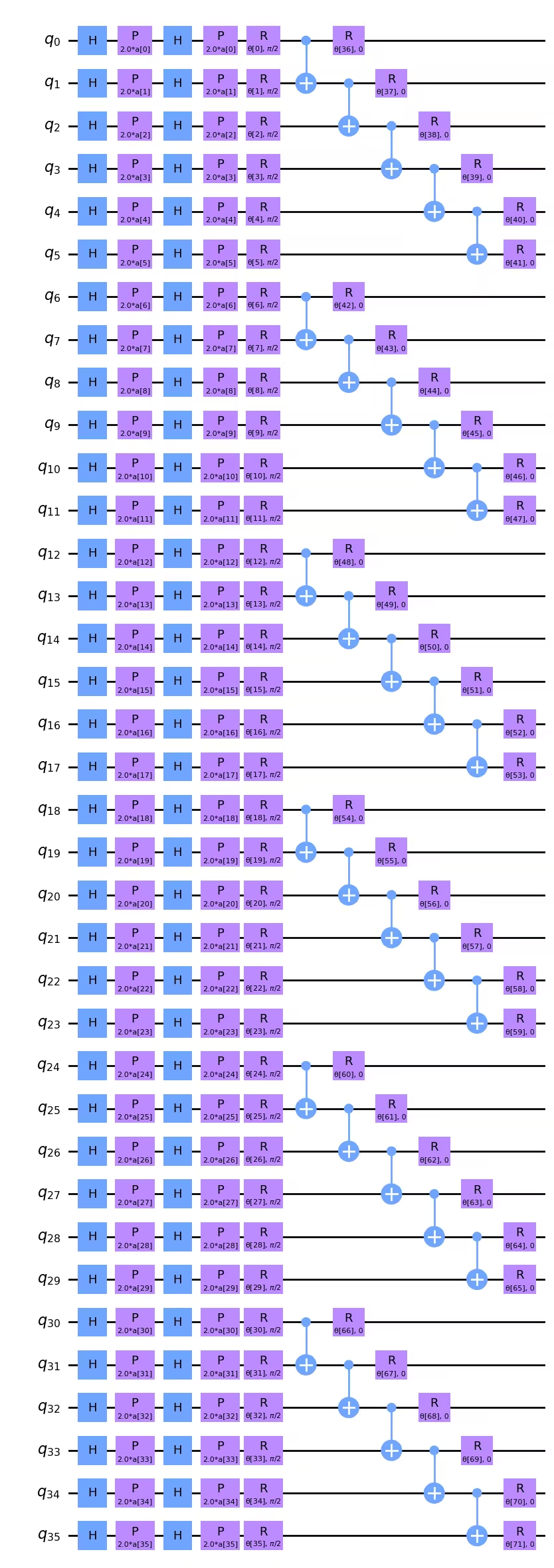
2量子ビット深さの最小化が最優先事項であれば、CNOTの順序を変えることで実際に少し削減できることに気づくかもしれません。例えば、 $q_{35}$ と $q_{34}$ 上のCNOTは上の回路図で左に移動でき、例えば $q_{30}$ と $q_{31}$ 上のCNOTの直下に配置できます。2量子ビットゲート深さ5の場合、トランスパイル後にこれが差を生むかどうかは明確ではありませんが、念頭に置いておく価値はあります。CNOTゲートの順序が対象の問題と論理的に一致することが重要な場合、ここでの深さは問題ありません。CNOTの順序が画像のデータ構造のモデリングに重要でない場合は、深さを最小化するためにこれらのCNOTゲートの順序を並べ替えるスクリプトを作成することもできます。

より大きな画像に対応するため、オブザーバブルも再定義する必要があります：

from qiskit.quantum_info import SparsePauliOp

observable = SparsePauliOp.from_list([("Z" * (num_qubits), 1)])

Qiskit Patternsステップ2：量子実行のために問題を最適化する

まず、実行に使用するバックエンドを選択します。ここでは、最もビジーでないバックエンドを使用します。

from qiskit_ibm_runtime import QiskitRuntimeService

# To run on hardware, select the least busy quantum computer or specify a particular one.
service = QiskitRuntimeService()
backend = service.least_busy(operational=True, simulator=False)
# backend = service.backend("ibm_brisbaneane")

print(backend.name)

ibm_brisbane

再び、最適化レベルを3に設定したパスマネージャーを定義します。

from qiskit.circuit.library import XGate
from qiskit.transpiler import PassManager
from qiskit.transpiler.passes import (
    ALAPScheduleAnalysis,
    ConstrainedReschedule,
    PadDynamicalDecoupling,
)
from qiskit.transpiler.preset_passmanagers import generate_preset_pass_manager

target = backend.target

pm = generate_preset_pass_manager(target=target, optimization_level=3)
pm.scheduling = PassManager(
    [
        ALAPScheduleAnalysis(target=target),
        ConstrainedReschedule(
            acquire_alignment=target.acquire_alignment,
            pulse_alignment=target.pulse_alignment,
            target=target,
        ),
        PadDynamicalDecoupling(
            target=target,
            dd_sequence=[XGate(), XGate()],
            pulse_alignment=target.pulse_alignment,
        ),
    ]
)

次に、パスマネージャーを複数回適用します。非常に広いまたは深い回路では、トランスパイル後の2量子ビット深さに大きなばらつきが生じることがあります。そのような回路では、パスマネージャーを何度も試して最良（最も浅い）結果を使用することが重要です。

# Try pass manager several times, since heuristics can return various transpilations on large circuits, and we want the shallowest.

transpiled_qcs = []
transpiled_depths = []
transpiled_2q_depths = []
for i in range(1, 10):
    circuit_ibm = pm.run(full_circuit)
    transpiled_qcs.append(circuit_ibm)
    transpiled_depths.append(circuit_ibm.decompose().depth())
    transpiled_2q_depths.append(
        circuit_ibm.decompose().depth(lambda instr: len(instr.qubits) > 1)
    )
    # print(i)

print(transpiled_depths)
print(transpiled_2q_depths)

# Use the shallowest

minpos = transpiled_2q_depths.index(min(transpiled_2q_depths))

[85, 85, 81, 89, 81, 81, 89, 85, 85]
[10, 10, 10, 10, 10, 10, 10, 10, 10]

この場合、トランスパイル後の2量子ビット深さは常に10であることがわかります。1量子ビット深さにわずかなばらつきがあり、最も浅いものを使用します。しかしこの36量子ビット回路では、これは重要な改善ではありません。このトランスパイルされた回路を可視化することはできますが、このスケールでは視覚的に解析することがますます困難になります。

circuit_ibm = transpiled_qcs[2]
observable_ibm = observable.apply_layout(circuit_ibm.layout)
print(circuit_ibm.decompose().depth())
print(
    f"2+ qubit depth: {circuit_ibm.decompose().depth(lambda instr: len(instr.qubits) > 1)}"
)

81
2+ qubit depth: 10

Qiskit Patternsステップ3：Qiskit Primitivesを使用して実行する

実際の量子コンピューターで使用する時間を制限するため、ここでは最適化ステップをわずかしか実行せず、非常に小さなトレーニングセットで行います。しかし、より多くの最適化ステップや大規模なテストデータセットへのスケーリングは、このレッスン全体の説明から明らかなはずです。

# This was run on an Eagle r3 processor on 10-4-24, and took 7 min.

from qiskit_ibm_runtime import EstimatorV2 as Estimator, Session

batch_size = 7
num_epochs = 1
num_samples = len(train_images)

# Globals
circuit = circuit_ibm
observable = observable_ibm
objective_func_vals = []
iter = 0

# Random initial weights for the ansatz
np.random.seed(42)
# weight_params = np.random.rand(len(ansatz.parameters)) * 2 * np.pi
# Or re-load weights from a previous calculation
weight_params = np.array(
    [
        3.35330497,
        5.97351416,
        4.59925358,
        3.76148219,
        0.98029403,
        0.98014248,
        0.3649501,
        6.44234523,
        3.77691701,
        4.44895122,
        0.12933619,
        6.09412333,
        5.23039137,
        1.33416598,
        1.14243996,
        1.15236452,
        1.91161039,
        3.2971419,
        3.71399059,
        1.82984665,
        3.84438512,
        0.87646578,
        1.83559896,
        2.30191935,
        2.86557222,
        4.93340606,
        1.25458737,
        3.23103027,
        3.72225051,
        0.29185655,
        3.81731689,
        1.07143467,
        0.40873121,
        5.96202367,
        6.067245,
        5.07931034,
        1.91394476,
        0.61369199,
        4.2991629,
        2.76555968,
        0.76678884,
        3.11128829,
        0.21606945,
        5.71342859,
        1.62596258,
        4.16275028,
        1.95853845,
        3.26768375,
        3.43508199,
        1.1614748,
        6.09207989,
        4.87030317,
        5.90304595,
        5.62236606,
        3.75671636,
        5.79230665,
        0.55601479,
        1.23139664,
        0.28417144,
        2.04411075,
        2.44213144,
        1.70493625,
        5.20711134,
        2.24154726,
        1.76516358,
        3.40986006,
        0.88545302,
        5.04035228,
        0.46841551,
        6.2007935,
        4.85215699,
        1.24856745,
    ]
)

# Running in a session avoids repeated queuing. This is available to Premium Plan, Flex Plan, and On-Prem (IBM Quantum Platform API) Plan users.

with Session(backend=backend) as session:
    estimator = Estimator(mode=session, options={"resilience_level": 1})

    for epoch in range(num_epochs):
        for i in range((num_samples - 1) // batch_size + 1):
            print(f"Epoch: {epoch}, batch: {i}")
            start_i = i * batch_size
            end_i = start_i + batch_size
            train_images_batch = np.array(train_images[start_i:end_i])
            train_labels_batch = np.array(train_labels[start_i:end_i])
            input_params = train_images_batch
            target = train_labels_batch
            iter = 0
            # We can increase maxiter to do a full optimization.
            res = minimize(
                mse_loss_weights,
                weight_params,
                method="COBYLA",
                options={"maxiter": 20},
            )
            weight_params = res["x"]
session.close()

# Open users can carry out the same calculation using a batch, but repeated queuing is possible.
# from qiskit_ibm_runtime import Batch

# with Batch(backend=backend) as batch:
#    estimator = Estimator(
#        mode=batch, options={"resilience_level": 1}
#    )
#
#    for epoch in range(num_epochs):
#        for i in range((num_samples - 1) // batch_size + 1):
#            print(f"Epoch: {epoch}, batch: {i}")
#            start_i = i * batch_size
#            end_i = start_i + batch_size
#            train_images_batch = np.array(train_images[start_i:end_i])
#            train_labels_batch = np.array(train_labels[start_i:end_i])
#            input_params = train_images_batch
#            target = train_labels_batch
#            iter = 0
#            # We can increase maxiter to do a full optimization.
#            res = minimize(
#                mse_loss_weights,
#                weight_params,
#                method="COBYLA",
#                options={"maxiter": 20},
#            )
#            weight_params = res["x"]
# batch.close()

この計算から返された重みパラメータは、さらなるイテレーションを行う場合に備えて保存することをお勧めします。

weight_params

array([3.35330497, 6.97351416, 5.59925358, 3.76148219, 0.98029403,
       0.98014248, 0.3649501 , 6.44234523, 3.77691701, 4.44895122,
       1.12933619, 7.09412333, 5.23039137, 1.33416598, 1.14243996,
       1.15236452, 1.91161039, 3.2971419 , 3.71399059, 1.82984665,
       3.84438512, 0.87646578, 1.83559896, 2.30191935, 2.86557222,
       4.93340606, 1.25458737, 3.23103027, 3.72225051, 0.29185655,
       3.81731689, 1.07143467, 0.40873121, 5.96202367, 6.067245  ,
       5.07931034, 1.91394476, 0.61369199, 4.2991629 , 2.76555968,
       0.76678884, 3.11128829, 0.21606945, 5.71342859, 1.62596258,
       4.16275028, 1.95853845, 3.26768375, 3.43508199, 1.1614748 ,
       6.09207989, 4.87030317, 5.90304595, 5.62236606, 3.75671636,
       5.79230665, 0.55601479, 1.23139664, 0.28417144, 2.04411075,
       2.44213144, 1.70493625, 5.20711134, 2.24154726, 1.76516358,
       3.40986006, 0.88545302, 5.04035228, 0.46841551, 6.2007935 ,
       4.85215699, 1.24856745])

最初の数回の最適化ステップをプロットできますが、わずかな最適化ステップの後には収束は期待できません。これらの曲線はシミュレーターを使用した場合でも、最初の数ステップでは比較的フラットです。ただし、現在の最適化には72個の自由パラメータがあることに注意が必要です。例えば、完全な行と列のサブセットに対応するデータで量子ビットをパラメータ化するなどの方法で、結果を損なうことなく少なくとも2〜3倍削減できます。実際、損失関数の最小化にさらなる量子計算時間を費やす前に、パラメータ空間を削減すべきです。

obj_func_vals_qc = objective_func_vals
# import matplotlib.pyplot as plt

plt.figure(figsize=(12, 6))
plt.plot(obj_func_vals_qc, label="revised ansatz")
plt.xlabel("iteration")
plt.ylabel("loss")
plt.legend()
plt.show()

Output of the previous code cell

まとめ

このレッスンでは、量子ニューラルネットワークを使った画像の二値分類のワークフローを学びました。Qiskitパターンの各ステップにおける主な考慮点は以下のとおりです。

ステップ1： 問題を量子回路にマッピングする

学習データを読み込む。これは「手動で」行うことも、z_feature_map のような事前構築済みの特徴マップを使用して行うこともできます。
問題に適した回転層とエンタングルメント層を含むアンザッツを構築する。
量子コンピューターで質の高い結果を得るために、回路の深さを監視する。

ステップ2： 量子実行のために問題を最適化する

バックエンドを選択する（多くの場合、最も混雑していないものを選ぶ）。
パスマネージャーを使用して、回路とオブザーバブルの両方を選択したバックエンドのアーキテクチャにトランスパイルする。
非常に深いまたは広い回路の場合は、複数回トランスパイルし、最も浅い回路を選択する。

ステップ3： Qiskit（Runtime）プリミティブを使って実行する

シミュレーターで事前試験を行い、アンザッツのデバッグと最適化を行う。
IBM®量子コンピューターで実行する。

ステップ4： 後処理を行い、結果を古典的な形式で返す

学習データおよびテストデータに対するモデルの精度を計算する。
古典的最適化の収束を監視する。

参考文献

[1] https://arxiv.org/abs/2405.00781

データ生成​

変分量子分類器：最初の試み​

Qiskitパターンのステップ1：問題を量子回路にマッピングする​

損失関数​

Qiskit Patterns ステップ2：量子実行に向けた問題の最適化​

Qiskit Patterns ステップ3：Qiskit Primitivesによる実行​

データセットをバッチ単位でループする​

Qiskit Patterns ステップ4：後処理と古典フォーマットでの結果返却​

テストと精度​

モデルの改善​

ステップ1の再考​

ステップ2の再考​

ステップ3の再考​

ステップ4の再考​

ステップ1：問題を量子回路にマッピングする​

Qiskit Patternsステップ2：量子実行のために問題を最適化する​

Qiskit Patternsステップ3：Qiskit Primitivesを使用して実行する​

まとめ​

参考文献​

データ生成

変分量子分類器：最初の試み

Qiskitパターンのステップ1：問題を量子回路にマッピングする

損失関数

Qiskit Patterns ステップ2：量子実行に向けた問題の最適化

Qiskit Patterns ステップ3：Qiskit Primitivesによる実行

データセットをバッチ単位でループする

Qiskit Patterns ステップ4：後処理と古典フォーマットでの結果返却

テストと精度

モデルの改善

ステップ1の再考

ステップ2の再考

ステップ3の再考

ステップ4の再考

ステップ1：問題を量子回路にマッピングする

Qiskit Patternsステップ2：量子実行のために問題を最適化する

Qiskit Patternsステップ3：Qiskit Primitivesを使用して実行する

まとめ

参考文献