確率的エラー増幅によるゼロノイズ外挿

ゼロノイズ外挿（ZNE）は、観測量の期待値計算における量子ノイズを軽減する手法です。量子回路をノイズ・スケールを上げながら実行し、それらのノイズ・スケールに対する期待値を取り、外挿してゼロノイズの期待値を推定します。ノイズ増幅と外挿の両段階は、さまざまな方法で実装できます。このガイドでは、"Evidence for the utility of quantum computing before fault tolerance"で提案されているように、確率的エラー増幅（PEA）でノイズを増幅します。PEAで増幅するには、まず回路のエンタングリング・ゲートに影響するノイズをモデル化する必要があります。ノイズ・モデルを必要としないデジタル・ゲート・フォールディングで増幅することもでき、ゲート・フォールディングのガイドで扱っています。ノイズはqiskit-noise-learningで学習し、組み込みの指数フィッティング戦略で外挿します。

ZNEは他の手法よりも低いサンプリング・コストで量子ノイズを軽減できますが、バイアスには上限がないことに注意してください。

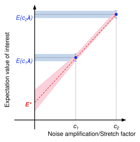
ワークフローは次のとおりです。

1. 回路と観測量を指定する
2. Qiskitのステートベクトル・シミュレーターを使って厳密な期待値を計算する
3. ノイズを含む、軽減されていない期待値を計算する
4. qiskit-noise-learning でエンタングリング層のノイズを学習する
5. 確率的エラー増幅によるZNEプログラムを準備し、ノイズ・スケールの異なる回路をサンプリングする
6. ゼロノイズ極限へ外挿する
7. 軽減された期待値を比較する

回路と観測量を指定する

このガイドでは、リング・トポロジーの8量子ビット上のトロッター化された横磁場イジング模型（TFIM）について、サイト平均磁化 $\langle Z \rangle_{\text{avg}} = \frac{1}{N} \sum_{i=1}^{N} \langle Z_i \rangle$ を計算します。横磁場の強さをいくつかの値でスイープし、磁化を磁場の強さの関数としてプロットします。偶数個の量子ビットからなるリング・トポロジーでは、下の結合マップに赤と緑で示すように、2量子ビット・ゲートの層を2つの固有な層に分割できます。ノイズ・モデルを学習したい場合は、固有な層が独立に学習される必要があるため、固有なエンタングリング層を最小限にした回路を設計することが重要です。回路に固有な層が多すぎると、多数の層を学習するためのサンプリング・コストにより、ノイズ学習が実行不可能になることがあります。

# Added by doQumentation — installs the packages this notebook needs if they are missing
import importlib.util

_needed = {"IPython": "IPython", "matplotlib": "matplotlib", "numpy": "numpy", "qiskit": "qiskit", "qiskit_aer": "qiskit-aer", "qiskit_ibm_runtime": "qiskit-ibm-runtime", "qiskit_mitigation": "qiskit-mitigation", "qiskit_noise_learning": "qiskit-noise-learning", "samplomatic": "samplomatic", "scipy": "scipy"}
_missing = [pip for module, pip in _needed.items()
            if importlib.util.find_spec(module) is None]
# One at a time, so a package that fails to install does not block the others
for _pip in _missing:
    %pip install -q {_pip}
if not _missing:
    print("\u2713 All required packages are installed")

import warnings

import IPython.display
import numpy as np
from qiskit.circuit import Parameter, QuantumCircuit
from qiskit.quantum_info import SparsePauliOp
from qiskit.visualization import plot_coupling_map

warnings.filterwarnings("ignore")

def trotter_circuit(num_qubits, theta, layers, num_steps):
    """Trotterized transverse-field Ising evolution: RX on every site, then a CZ layer per coupling layer."""
    circuit = QuantumCircuit(num_qubits)
    for _ in range(num_steps):
        circuit.rx(theta, range(num_qubits))
        for layer in layers:
            circuit.barrier()
            for edge in layer:
                circuit.cz(*edge)
                circuit.sdg(edge)
            circuit.barrier()
    return circuit

num_qubits = 8
trotter_steps = 15
ring_coupling = [(i, (i + 1) % num_qubits) for i in range(num_qubits)]
layers = [
    ring_coupling[0::2],
    ring_coupling[1::2],
]  # two disjoint layers of CZ gates
theta = Parameter("theta")
circuit = trotter_circuit(num_qubits, theta, layers, trotter_steps)

# Parameter values: theta in [0, 0.25 pi] - values for the transverse-field sweep
data_points = 6
parameter_values = np.linspace(0, 0.25 * np.pi, data_points).reshape(
    (data_points, 1)
)

# Define observables - Z on each site
observables = [
    SparsePauliOp("I" * (num_qubits - q - 1) + "Z" + "I" * q)
    for q in range(num_qubits)
]

print("Edges of the same color may execute their gates simultaneously.")
IPython.display.display(
    plot_coupling_map(
        num_qubits=num_qubits,
        qubit_coordinates=None,
        coupling_map=ring_coupling,
        figsize=(4, 4),
        qubit_size=150,
        line_width=5,
        line_color=[
            "red" if edge in layers[0] else "green" for edge in ring_coupling
        ],
        font_size=90,
    )
)
print("Visualization of 1 Trotter step")
trotter_circuit(num_qubits, theta, layers, 1).draw("mpl", scale=0.7)

Edges of the same color may execute their gates simultaneously.

Visualization of 1 Trotter step

Qiskitのステートベクトル・シミュレーターを使って厳密な期待値を計算する

Qiskitの Statevector クラスを使用して、$\theta$ の各値について各サイトでの $Z_i$ の厳密な期待値を計算します。

from qiskit.quantum_info import Statevector
import matplotlib.pyplot as plt

exact_evs = np.array(
    [
        [
            Statevector(circuit.assign_parameters([value]))
            .expectation_value(obs)
            .real
            for value in parameter_values.ravel()
        ]
        for obs in observables
    ]
)  # shape (observables, parameter values)

x_vals = parameter_values.ravel() / np.pi
fig, ax = plt.subplots(figsize=(7, 4))
ax.plot(x_vals, exact_evs.mean(axis=0), "ko-", label="Exact")
ax.set_xlabel(r"$\theta/\pi$")
ax.set_ylabel(r"$\langle Z \rangle_{\text{avg}}$")
ax.legend()
plt.tight_layout()
plt.show()

ノイズを含む、軽減されていない期待値を計算する

QuantumProgram は、Executorプリミティブに適した形式で、量子回路とsamplexを含みます。MitigationTask.prepare は、回路、観測量、パラメーター値から QuantumProgram を構築し、指定されたボクシング・オプションで回路をボックス化します。measure_annotations ボクシング・オプションを "change_basis" に設定して測定を必要な基底に回転させ、さらに add_tags: "unique_box" を追加して、シミュレーターがノイズ・モデルを回路のボックスにマッピングできるようにします。プログラムはデフォルトでパウリ・ツワーリングされ、ハードウェア上ではコヒーレント・ノイズが、軽減手法が想定するパウリ・ノイズに変換されます。num_randomizations は各回路についてサンプリングするツワーリング済みインスタンスの数を、shots_per_randomization は各インスタンスが受け取るショット数を設定するため、それらの積が回路あたりのショット予算になります。

QPUにアクセスできるユーザーは、QiskitRuntimeService のバックエンドから構築した Executor でプログラムを実行します。ここでは AerSimulator を Executor に渡してプログラムをローカルで実行し、そのシミュレーターオプション layer_noise_model を使って、エンタングリングゲートのすべてのレイヤーにランダムなPauli-Lindbladノイズモデルを注入します。このモデルは qiskit-mitigation の random_pauli_lindblad_noise で生成し、レイヤーゲートあたりのエラー(EPLG)を現在のHeron QPUに典型的な 0.003 としています。

from qiskit.circuit import CircuitInstruction
from qiskit.quantum_info import PauliLindbladMap, pauli_basis
from qiskit_aer import AerSimulator
from qiskit_ibm_runtime import Executor
from qiskit_mitigation import MitigationTask, find_combined_unique_layers

def generate_random_pauli_lindblad_noise(
    layers,
    num_qubits: int,
    eplg: float = 3e-3,
    seed: int | None = None,
) -> list[tuple[CircuitInstruction, PauliLindbladMap]]:
    """Generate random Pauli-Lindblad noise over the full Pauli basis."""
    layer_noise_model = []
    for layer in layers:
        layer_instructions = layer.operation.params[0]
        contain_measurement = any(
            inst.name.startswith("measure") for inst in layer_instructions
        )
        if contain_measurement:  # do not add measurement noise
            layer_noise = PauliLindbladMap.identity(num_qubits)
        else:
            edges = [
                (inst.qubits[0]._index, inst.qubits[1]._index)
                for inst in layer_instructions
            ]  # extract the edges of the layer

            basis_paulis = [p for p in pauli_basis(2) if np.sum(p.x + p.z)]
            rng = np.random.default_rng(seed=seed)
            num_generators = len(basis_paulis)
            rates = rng.random(len(basis_paulis)) * eplg / num_generators

            layer_noise = PauliLindbladMap.from_sparse_list(
                [
                    (pauli.to_label(), edge, rate)
                    for pauli, rate in zip(basis_paulis, rates, strict=True)
                    for edge in edges
                ],
                num_qubits=num_qubits,
            )
        layer_noise_model.append((layer, layer_noise))
    return layer_noise_model

num_randomizations = 50
shots_per_randomization = 64

boxing_options = {
    "measure_annotations": "change_basis",
    "add_tags": "unique_box",
}

# find the unique layers to generate the layered noise for
box_layers = find_combined_unique_layers(
    [circuit], custom_boxing_options=boxing_options
)
layer_noise_model = generate_random_pauli_lindblad_noise(
    box_layers, num_qubits, seed=42
)

# a local noisy simulator in place of a QPU backend
noisy_executor = Executor(
    AerSimulator(),
    options={"simulator": {"layer_noise_model": layer_noise_model}},
)

task = MitigationTask()
program = task.prepare(
    circuit=circuit,
    observables=observables,
    parameters=parameter_values,
    num_randomizations=num_randomizations,
    shots_per_randomization=shots_per_randomization,
    custom_boxing_options=boxing_options,
)
program._semantic_role = "simulation"  # flag the program for the simulator
unmitigated_res = task.postprocess(noisy_executor.run(program).result())

fig, ax = plt.subplots(figsize=(7, 4))
ax.plot(x_vals, exact_evs.mean(axis=0), "k-", label="Exact")
ax.errorbar(
    x_vals,
    np.mean(unmitigated_res.data.evs, axis=0),
    np.mean(unmitigated_res.data.stds, axis=0),
    fmt="o-",
    label="Unmitigated",
)
ax.set_xlabel(r"$\theta/\pi$")
ax.set_ylabel(r"$\langle Z \rangle_{\text{avg}}$")
ax.legend()
plt.tight_layout()
plt.show()

qiskit-noise-learning でエンタングリングレイヤーのノイズを学習する

PEAは、回路内の各エンタングリングゲートのレイヤーについて、ツワール化されたノイズモデルを学習することから始まります。マルコフ型のノイズモデルを仮定するため、回路の深さは特定のエンタングリングレイヤーのノイズチャネルに影響しないと想定され、一意なエンタングリングゲートのレイヤーごとにノイズモデルを学習するだけで済みます。学習したノイズモデルが正確であるほど、増幅もより正確になります。

ノイズの学習には qiskit-noise-learning を使用します。学習器は学習用回路内で各レイヤーを fragment_depths 回繰り返し、各回路を num_randomizations 回ツワール化し、測定された忠実度の減衰をPauli-Lindbladモデルにフィットさせます。次のコードは、2つのレイヤーを1つのマップにまとめた学習済みノイズモデルを描画します。各量子ビットは、2つのレイヤーにわたって合計した重み1のX、Y、Zレートの円グラフで表され、各エッジは学習した重み2のレートを示します。3e-4 というレートは、そのレイヤーを10,000回使用するうちおよそ3回その誤りが発生することを意味します。

from qiskit.providers.fake_provider import GenericBackendV2
from qiskit.quantum_info import PauliList
from qiskit_ibm_runtime.results import LayerError, PauliLindbladError
from qiskit_ibm_runtime.visualization.embeddings import Embedding
from qiskit_mitigation import PEA
from qiskit_noise_learning.aer_executor import AerExecutor
from qiskit_noise_learning.noise_learner import LearningOptions, NoiseLearner
from samplomatic import InjectNoise, Tag
from samplomatic.utils import get_annotation

backend = GenericBackendV2(
    num_qubits=num_qubits,
    basis_gates=["id", "rz", "sx", "x", "cz"],
    coupling_map=ring_coupling,
)

task_pea = PEA()
# learn only the layers PEA will inject noise into, i.e. not the measurement layer
pea_layers = [
    layer
    for layer in task_pea.find_unique_layers(circuit, boxing_options)
    if get_annotation(layer.operation, InjectNoise)
]

learning_options = LearningOptions(
    fragment_depths=[2, 4, 8, 16],
    num_randomizations=50,
    shots_per_randomizations=64,
)
# qiskit-noise-learning is not compatible with the Executor in local mode,
# and requires the simulator present in the package for running simulation
noise_dict = {
    get_annotation(layer.operation, Tag).ref: noise_layer
    for layer, noise_layer in layer_noise_model
}
noise_learner_simulator = AerExecutor(
    qasm_simulator=AerSimulator(), noise_dict=noise_dict
)
learner = NoiseLearner(
    backend, options=learning_options, executor=noise_learner_simulator
)
learned_noise = (
    learner.run(pea_layers).result().to_dict()
)  # keyed by InjectNoise reference

# Draw the learned model on the ring, laid out as a square with the qubits in ring order.
# Composing the two layers' maps sums their rates, giving one map over all the ring's edges.
embedding = Embedding(
    [(0, 0), (0, 2), (0, 4), (2, 4), (4, 4), (4, 2), (4, 0), (2, 0)],
    ring_coupling,
)
first, second = learned_noise.values()
learned_model = first.compose(second).simplify()
error = PauliLindbladError(
    PauliList(
        learned_model.get_qubit_sparse_pauli_list_copy().to_pauli_list()
    ),
    learned_model.rates,
)
fig = LayerError(circuit, list(range(num_qubits)), error).draw_map(
    embedding, radius=0.4, height=460, width=620
)
fig.update_traces(
    marker={
        "cmin": 0,
        "cmax": max(learned_model.rates),
        "colorbar": {"tickformat": ".1e", "title": "rate"},
    },
    selector={"mode": "markers"},
)
fig.show()

確率的エラー増幅を用いたZNEプログラムを準備し、異なるノイズスケールの回路をサンプリングする

ここでは、ノイズスケールが増加していく回路を含むZNEプログラムを準備します。PEAでは、各ノイズ係数は回路が受ける学習済みノイズの倍数を表します。2.0 というノイズ係数は、レイヤーがもともと持っているノイズに加えて、そのレイヤーの後に各レイヤーの学習済みノイズチャネルをもう1つ分注入します。PEAはゲートを繰り返すのではなく学習したノイズレートを直接スケールするため、整数でないものを含め任意のノイズ係数が可能で、回路自体は変更されません。プログラムの各項目は1つのテンプレート回路を共有し、samplexが注入するノイズだけが異なります。注入されるノイズはランダム化ごとに1回サンプリングされるため、PEAの統計誤差はランダム化あたりのショット数ではなくランダム化の回数で制御されます。そのため、少数のショットで多数のランダム化を行い、総ショット数を未軽減のプログラムと同じに保ちます。ランダム化の回数が少なすぎないようにすることが重要です。そうしないと、ノイズ注入にサンプリングバイアスが生じる可能性があります。

サンプリングオーバーヘッドの合計は、ノイズ係数の数に比例して増加します。

noise_factors = [1, 2, 3]
program_pea = task_pea.prepare(
    circuit=circuit,
    observables=observables,
    parameters=parameter_values,
    num_randomizations=200,
    shots_per_randomization=16,
    custom_boxing_options=boxing_options,
    noise_maps=learned_noise,
    noise_factors=noise_factors,
)

最後に、ノイズのあるシミュレーターでプログラムを実行します。その結果は次のステップの外挿に使われます。

program_pea._semantic_role = (
    "simulation"  # flag the program for the simulator
)
job_pea_results = noisy_executor.run(program_pea).result()

ゼロノイズ極限へ外挿する

各ノイズスケールのデータが得られたので、データに関数をフィットさせ、ゼロノイズ値まで外挿し戻すことで、ノイズのない観測量の期待値を推定できます。Pauliノイズの下では、観測量はノイズ係数に対して指数関数的に減衰するため、最初の選択肢として指数外挿器を選び、指数フィットが失敗した場合は線形外挿器にフォールバックします。外挿を可視化するために、各ノイズ係数で計算したサイト平均磁化、指数フィット、およびゼロノイズ点における外挿された期待値のサイト平均をプロットします。この特定の観測量では、フィットがやや過小評価していることがわかります。

from scipy.optimize import curve_fit

pea_mitigated_res = task_pea.postprocess(
    job_pea_results, extrapolator=["exponential", "linear"]
)

# The result holds the expectation value at each noise factor and the extrapolated value for
# every observable; we average them over the sites and fit the same model to draw the curve.
angle = 3  # theta = 0.15 pi, the angle with the largest unmitigated error
amplifications = pea_mitigated_res.data.evs_noise_factors[:, angle, :].mean(
    axis=0
)
x_fit = np.linspace(0, max(noise_factors), 51)
params, _ = curve_fit(
    lambda x, a, b: a * np.exp(b * x),
    noise_factors,
    amplifications,
    p0=[1.0, -0.1],
)

plt.plot(
    noise_factors, amplifications, "o", color="red", label="amplifications"
)
plt.plot(
    x_fit,
    params[0] * np.exp(params[1] * x_fit),
    "--",
    color="black",
    label="exponential fit",
)
plt.plot(
    [0],
    pea_mitigated_res.data.evs[:, angle].mean(),
    "*",
    color="black",
    markersize=15,
    label="extrapolation",
)
plt.plot(
    [0],
    exact_evs[:, angle].mean(),
    "_",
    color="red",
    markersize=15,
    markeredgewidth=3,
    label="exact",
)
plt.xlabel("noise factor")
plt.ylabel(r"$\langle Z \rangle_{\text{avg}}$")
plt.legend()
plt.show()

軽減された期待値を比較する

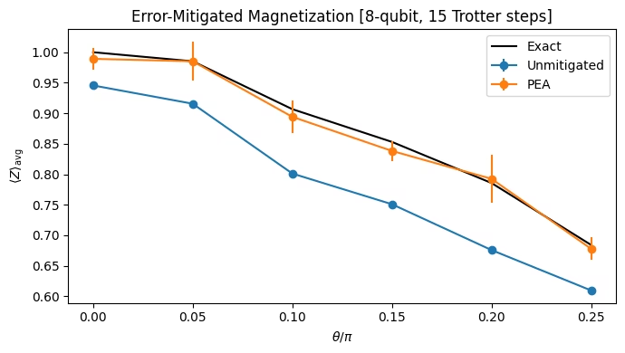
イジング回転角のスイープ全体で、各手法のサイト平均磁化をプロットします。PEAは誤差範囲内で正確な磁化を回復しますが、未軽減の結果は大きく下方にずれています。

results = {
    "Unmitigated": unmitigated_res,
    "PEA": pea_mitigated_res,
}

fig, ax = plt.subplots(figsize=(7, 4))
ax.plot(x_vals, exact_evs.mean(axis=0), "k-", label="Exact")
for label, res in results.items():
    ax.errorbar(
        x_vals,
        np.mean(res.data.evs, axis=0),
        np.mean(res.data.stds, axis=0),
        fmt="o-",
        label=label,
    )
ax.set_xlabel(r"$\theta/\pi$")
ax.set_ylabel(r"$\langle Z \rangle_{\text{avg}}$")
ax.legend()
ax.set_title(
    f"Error-Mitigated Magnetization [{num_qubits}-qubit, {trotter_steps} Trotter steps]"
)
plt.tight_layout()
plt.show()