ゲート・フォールディングとカスタム外挿によるゼロノイズ外挿

ゼロノイズ外挿（ZNE）は、観測量の期待値計算における量子ノイズを軽減する手法です。量子回路をノイズ・スケールを上げながら実行し、それらのノイズ・スケールに対する期待値を取り、外挿してゼロノイズの期待値を推定します。ノイズ増幅と外挿の両段階は、さまざまな方法で実装できます。このガイドでは、「デジタル・ゲート・フォールディング」でノイズを増幅します。これは、2量子ビット・ゲートを、そのゲートとその逆ゲートからなる等価な系列に置き換えることを意味します。例えば、ユニタリー $U$ を $U U^† U$ に置き換えると、ノイズ増幅係数は3になります。確率的エラー増幅（PEA）で増幅することもできます。これにはノイズ・モデルを学習する追加のステップが必要で、確率的エラー増幅のガイドで扱っています。このガイドでは、組み込みのフィッティング戦略（線形と指数）をいくつか使って外挿し、独自のカスタム・フィッティング関数を実装する方法も示します。

ZNEは他の手法よりも低いサンプリング・コストで量子ノイズを軽減できますが、バイアスには上限がないことに注意してください。

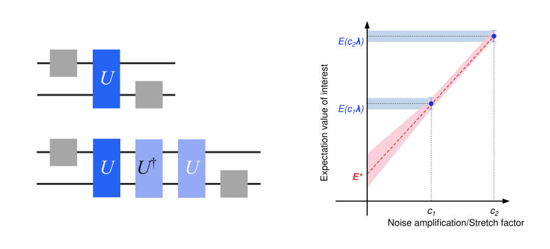
ワークフローは次のとおりです。

1. 回路と観測量を指定する
2. Qiskitのステートベクトル・シミュレーターを使って厳密な期待値を計算する
3. ノイズを含む、軽減されていない期待値を計算する
4. デジタル・ゲート・フォールディングによるZNEプログラムを準備し、ノイズ・スケールの異なる回路をサンプリングする
5. 組み込みおよびカスタムのフィッティング関数でゼロノイズ極限へ外挿する
6. 軽減された期待値を比較する

回路と観測量を指定する

リング・トポロジーの8量子ビット上のトロッター化された横磁場イジング模型（TFIM）について、サイト平均磁化 $\langle Z \rangle_{\text{avg}} = \frac{1}{N} \sum_{i=1}^{N} \langle Z_i \rangle$ を計算します。横磁場の強さをいくつかの値でスイープし、磁化を磁場の強さの関数としてプロットします。

# Added by doQumentation — installs the packages this notebook needs if they are missing
import importlib.util

_needed = {"IPython": "IPython", "matplotlib": "matplotlib", "numpy": "numpy", "qiskit": "qiskit", "qiskit_aer": "qiskit-aer", "qiskit_ibm_runtime": "qiskit-ibm-runtime", "qiskit_mitigation": "qiskit-mitigation", "scipy": "scipy"}
_missing = [pip for module, pip in _needed.items()
            if importlib.util.find_spec(module) is None]
# One at a time, so a package that fails to install does not block the others
for _pip in _missing:
    %pip install -q {_pip}
if not _missing:
    print("\u2713 All required packages are installed")

import warnings

import numpy as np
from qiskit.circuit import Parameter, QuantumCircuit
from qiskit.quantum_info import SparsePauliOp

warnings.filterwarnings("ignore")

def trotter_circuit(num_qubits, theta, layers, num_steps):
    """Trotterized transverse-field Ising evolution: RX on every site, then a CZ layer per coupling layer."""
    circuit = QuantumCircuit(num_qubits)
    for _ in range(num_steps):
        circuit.rx(theta, range(num_qubits))
        for layer in layers:
            circuit.barrier()
            for edge in layer:
                circuit.cz(*edge)
                circuit.sdg(edge)
            circuit.barrier()
    return circuit

num_qubits = 8
trotter_steps = 15
ring_coupling = [(i, (i + 1) % num_qubits) for i in range(num_qubits)]
layers = [
    ring_coupling[0::2],
    ring_coupling[1::2],
]  # two disjoint layers of CZ gates
theta = Parameter("theta")
circuit = trotter_circuit(num_qubits, theta, layers, trotter_steps)

# Parameter values: theta in [0, 0.25 pi] - values for the transverse-field sweep
data_points = 6
parameter_values = np.linspace(0, 0.25 * np.pi, data_points).reshape(
    (data_points, 1)
)

# Define observables - Z on each site
observables = [
    SparsePauliOp("I" * (num_qubits - q - 1) + "Z" + "I" * q)
    for q in range(num_qubits)
]

print("Visualization of 1 Trotter step")
trotter_circuit(num_qubits, theta, layers, 1).draw("mpl", scale=0.7)

Visualization of 1 Trotter step

Qiskitのステートベクトル・シミュレーターを使って厳密な期待値を計算する

Qiskitの Statevector クラスを使用して、$\theta$ の各値について各サイトでの $Z_i$ の厳密な期待値を計算します。

import matplotlib.pyplot as plt
from qiskit.quantum_info import Statevector

exact_evs = np.array(
    [
        [
            Statevector(circuit.assign_parameters([value]))
            .expectation_value(obs)
            .real
            for value in parameter_values.ravel()
        ]
        for obs in observables
    ]
)  # shape (observables, parameter values)

x_vals = parameter_values.ravel() / np.pi
fig, ax = plt.subplots(figsize=(7, 4))
ax.plot(x_vals, exact_evs.mean(axis=0), "ko-", label="Exact")
ax.set_xlabel(r"$\theta/\pi$")
ax.set_ylabel(r"$\langle Z \rangle_{\text{avg}}$")
ax.legend()
plt.tight_layout()
plt.show()

ノイズを含む、軽減されていない期待値を計算する

QuantumProgram は、Executorプリミティブに適した形式で、量子回路とsamplexを含みます。MitigationTask.prepare は、回路、観測量、パラメーター値から QuantumProgram を構築し、指定されたボクシング・オプションで回路をボックス化します。measure_annotations ボクシング・オプションを "change_basis" に設定して測定を必要な基底に回転させ、さらに add_tags: "unique_box" を追加して、シミュレーターがノイズ・モデルを回路のボックスにマッピングできるようにします。プログラムはデフォルトでパウリ・ツワーリングされ、ハードウェア上ではコヒーレント・ノイズが、軽減手法が想定するパウリ・ノイズに変換されます。num_randomizations は各回路についてサンプリングするツワーリング済みインスタンスの数を、shots_per_randomization は各インスタンスが受け取るショット数を設定するため、それらの積が回路あたりのショット予算になります。

QPUにアクセスできるユーザーは、QiskitRuntimeService のバックエンドから構築した Executor でプログラムを実行します。ここでは、プログラムをローカルで実行する AerSimulator を Executor に渡し、そのシミュレーター・オプション layer_noise_model を使って、エンタングリング・ゲートのすべての層にランダムなパウリ・リンドブラッド・ノイズ・モデルを注入します。このモデルは qiskit-mitigation の random_pauli_lindblad_noise で生成し、層ゲートあたりのエラー（EPLG）は現在のHeron QPUに典型的な 0.003 とします。

from qiskit.circuit import CircuitInstruction
from qiskit.quantum_info import PauliLindbladMap, pauli_basis
from qiskit_aer import AerSimulator
from qiskit_ibm_runtime import Executor
from qiskit_mitigation import MitigationTask, find_combined_unique_layers

def generate_random_pauli_lindblad_noise(
    layers,
    num_qubits: int,
    eplg: float = 3e-3,
    seed: int | None = None,
) -> list[tuple[CircuitInstruction, PauliLindbladMap]]:
    """Generate random Pauli-Lindblad noise over the full Pauli basis."""
    layer_noise_model = []
    for layer in layers:
        layer_instructions = layer.operation.params[0]
        contain_measurement = any(
            inst.name.startswith("measure") for inst in layer_instructions
        )
        if contain_measurement:  # do not add measurement noise
            layer_noise = PauliLindbladMap.identity(num_qubits)
        else:
            edges = [
                (inst.qubits[0]._index, inst.qubits[1]._index)
                for inst in layer_instructions
            ]  # extract the edges of the layer

            basis_paulis = [p for p in pauli_basis(2) if np.sum(p.x + p.z)]
            rng = np.random.default_rng(seed=seed)
            num_generators = len(basis_paulis)
            rates = rng.random(len(basis_paulis)) * eplg / num_generators

            layer_noise = PauliLindbladMap.from_sparse_list(
                [
                    (pauli.to_label(), edge, rate)
                    for pauli, rate in zip(basis_paulis, rates, strict=True)
                    for edge in edges
                ],
                num_qubits=num_qubits,
            )
        layer_noise_model.append((layer, layer_noise))
    return layer_noise_model

num_randomizations = 50
shots_per_randomization = 64

boxing_options = {
    "measure_annotations": "change_basis",
    "add_tags": "unique_box",
}

# find the unique layers to generate the layered noise for
box_layers = find_combined_unique_layers(
    [circuit], custom_boxing_options=boxing_options
)
layer_noise_model = generate_random_pauli_lindblad_noise(
    box_layers, num_qubits, seed=42
)

# a local noisy simulator in place of a QPU backend
noisy_executor = Executor(
    AerSimulator(),
    options={"simulator": {"layer_noise_model": layer_noise_model}},
)

task = MitigationTask()
program = task.prepare(
    circuit=circuit,
    observables=observables,
    parameters=parameter_values,
    num_randomizations=num_randomizations,
    shots_per_randomization=shots_per_randomization,
    custom_boxing_options=boxing_options,
)
program._semantic_role = "simulation"  # flag the program for the simulator
unmitigated_res = task.postprocess(noisy_executor.run(program).result())

fig, ax = plt.subplots(figsize=(7, 4))
ax.plot(x_vals, exact_evs.mean(axis=0), "k-", label="Exact")
ax.errorbar(
    x_vals,
    np.mean(unmitigated_res.data.evs, axis=0),
    np.mean(unmitigated_res.data.stds, axis=0),
    fmt="o-",
    label="Unmitigated",
)
ax.set_xlabel(r"$\theta/\pi$")
ax.set_ylabel(r"$\langle Z \rangle_{\text{avg}}$")
ax.legend()
plt.tight_layout()
plt.show()

デジタル・ゲート・フォールディングによるZNEプログラムを準備し、ノイズ・スケールの異なる回路をサンプリングする

ノイズ・スケールを上げた回路を含むZNEプログラムを準備します。各ノイズ係数は、回路に含まれるエンタングリング・ゲートの倍数を表します（ノイズ係数 3.0 の回路は、元の回路の3倍のエンタングリング・ゲートを含みます）。各ノイズ係数の回路は、軽減されていないプログラムと同じ数のランダム化とショットでツワーリングされます。

from qiskit_mitigation import GateFolding

task_gf = GateFolding()
program_zne = task_gf.prepare(
    circuit=circuit,
    observables=observables,
    parameters=parameter_values,
    num_randomizations=num_randomizations,
    shots_per_randomization=shots_per_randomization,
    custom_boxing_options=boxing_options,
    noise_factors=[1, 3, 5],  # ZNE option
)

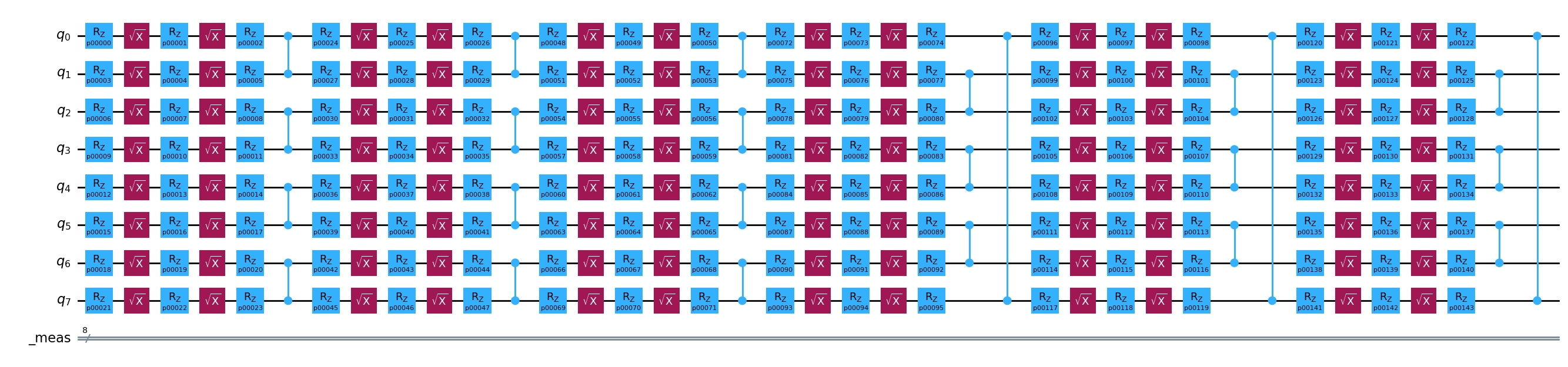
増幅を可視化するために、ツワーリング済みテンプレートの最初のトロッター・ステップを、ノイズ係数1とノイズ係数3で描画します。ノイズ係数3.0では、回路のすべての層が、その層、その逆、そして再びその層に置き換えられます。

import IPython.display

def first_trotter_step(template, noise_factor):
    """The template up to the closing barrier of its first Trotter step (two layers, each folded ``noise_factor`` times)."""
    toy = template.copy_empty_like()
    for instruction in template.data:
        toy.append(instruction)
        if (
            instruction.operation.name == "barrier"
            and instruction.operation.label.startswith(
                f"R{2 * noise_factor - 1}@"
            )
        ):
            break
    return toy

IPython.display.display(
    first_trotter_step(program_zne.items[0].circuit, 1).draw(
        "mpl", scale=0.7, plot_barriers=False
    )
)
first_trotter_step(program_zne.items[1].circuit, 3).draw(
    "mpl", fold=-1, plot_barriers=False
)

最後に、ノイズのあるシミュレーター上でプログラムを実行します。その結果は、次のステップの外挿に使われます。

program_zne._semantic_role = (
    "simulation"  # flag the program for the simulator
)
job_zne_results = noisy_executor.run(program_zne).result()

組み込みおよびカスタムのフィッティング関数でゼロノイズ極限へ外挿する

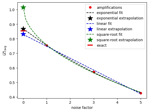
各ノイズ・スケールのデータが得られたので、そのデータに関数をフィッティングし、ゼロノイズの値まで外挿して、ノイズのない観測量の期待値を推定できます。データをフィッティングする方法は多数あり、適切な関数の選択はサンプリングされるデータの性質に依存します。GateFolding.postprocess は、linear、exponential、double_exponential を含む、いくつかの組み込み外挿関数を提供します。postprocess メソッドは外挿手法のリストを受け取り、それらを順に評価して、物理的に妥当な値で分散が有限である最初の値を返します。つまり、外挿器を指定する順序が、どの外挿器が選ばれるかに大きく影響します。外挿器として fallback を渡すと、有効な答えが見つからなかった場合に、最小のノイズ係数の期待値が選ばれて返されます。fallback が渡されておらず、物理的に妥当な値を返す外挿器がない場合は、std が最小の結果が返されます。パウリ・ノイズの下では、観測量はノイズ係数とともに指数関数的に減衰するため、エンタングリング・ゲートが30層（15トロッター・ステップ、1ステップあたり2層）ある場合、指数外挿器が自然な選択です。減衰が小さい場合によく選ばれる線形外挿も使えます。

カスタム・フィッティング関数を使うには、"custom" 外挿器を、フィッティング関数、各パラメーターの初期推定値のリスト、そして境界を含む custom_fit タプルと一緒に渡します。これらは scipy.optimize.curve_fit に転送されます。ポストプロセスは、プログラムを再実行せずに、異なる外挿器で繰り返すことができます。ここでは、カスタムの平方根フィッティング関数を使用します。外挿を可視化するために、$\theta = 0.15\pi$ について各ノイズ係数で計算したサイト平均磁化、3つのフィット、そしてゼロノイズ点での外挿された期待値のサイト平均をプロットします。3つのデータ点はほぼ線形に見えますが、線形外挿は厳密値より明らかに低い値になります。予想どおり、指数フィットがノイズのない期待値を最も効果的に推定します。

from scipy.optimize import curve_fit

zne_mitigated_exp = task_gf.postprocess(
    job_zne_results, extrapolator=["exponential", "linear"]
)
zne_mitigated_lin = task_gf.postprocess(
    job_zne_results, extrapolator=["linear"]
)

def sqrt_fit(x, a, b):
    return a * np.sqrt(x) + b

custom_fit = (sqrt_fit, [1.0, 1.0], (-np.inf, np.inf))
zne_mitigated_custom = task_gf.postprocess(
    job_zne_results,
    extrapolator=["custom", "exponential", "linear"],
    custom_fit=custom_fit,
)

# The result holds the expectation value at each noise factor and the extrapolated value, but
# not the fit parameters, so we refit the same models here to draw the curves.
noise_factors = np.array([1, 3, 5])
angle = 3  # theta = 0.15 pi, the angle with the largest unmitigated error
amplifications = zne_mitigated_exp.data.evs_noise_factors[:, angle, :].mean(
    axis=0
)
x_fit = np.linspace(0, 5, 51)
fits = {
    "exponential": (
        lambda x, a, b: a * np.exp(b * x),
        zne_mitigated_exp,
        "black",
    ),
    "linear": (lambda x, a, b: a * x + b, zne_mitigated_lin, "blue"),
    "square-root": (sqrt_fit, zne_mitigated_custom, "green"),
}

plt.plot(
    noise_factors, amplifications, "o", color="red", label="amplifications"
)
for name, (fit, res, color) in fits.items():
    params, _ = curve_fit(fit, noise_factors, amplifications, p0=[1.0, -0.1])
    plt.plot(
        x_fit, fit(x_fit, *params), "--", color=color, label=f"{name} fit"
    )
    plt.plot(
        [0],
        res.data.evs[:, angle].mean(),
        "*",
        color=color,
        markersize=15,
        label=f"{name} extrapolation",
    )
plt.plot(
    [0],
    exact_evs[:, angle].mean(),
    "_",
    color="red",
    markersize=15,
    markeredgewidth=3,
    label="exact",
)
plt.xlabel("noise factor")
plt.ylabel(r"$\langle Z \rangle_{\text{avg}}$")
plt.legend()
plt.show()

軽減された期待値を比較する

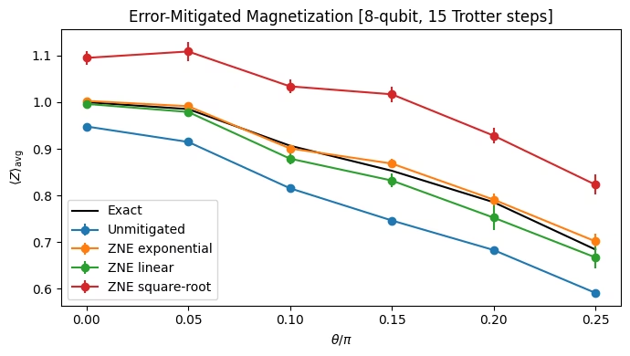
イジング回転角のスイープ全体にわたって、各手法のサイト平均磁化をプロットします。指数外挿は誤差範囲内で厳密な磁化を回復します。一方、線形外挿はバイアスの多くを取り除きますが、真の減衰が指数関数的であるため、一貫して過小評価します。平方根フィットはひどく過大評価します。

results = {
    "Unmitigated": unmitigated_res,
    "ZNE exponential": zne_mitigated_exp,
    "ZNE linear": zne_mitigated_lin,
    "ZNE square-root": zne_mitigated_custom,
}

fig, ax = plt.subplots(figsize=(7, 4))
ax.plot(x_vals, exact_evs.mean(axis=0), "k-", label="Exact")
for label, res in results.items():
    ax.errorbar(
        x_vals,
        np.mean(res.data.evs, axis=0),
        np.mean(res.data.stds, axis=0),
        fmt="o-",
        label=label,
    )
ax.set_xlabel(r"$\theta/\pi$")
ax.set_ylabel(r"$\langle Z \rangle_{\text{avg}}$")
ax.legend()
ax.set_title(
    f"Error-Mitigated Magnetization [{num_qubits}-qubit, {trotter_steps} Trotter steps]"
)
plt.tight_layout()
plt.show()