論理ノイズモデルを用いた確率的エラーキャンセレーション
使用量の目安: Heron r3 プロセッサーで28分。(注: これはあくまで目安であり、実際の実行時間は変動する場合があります。)
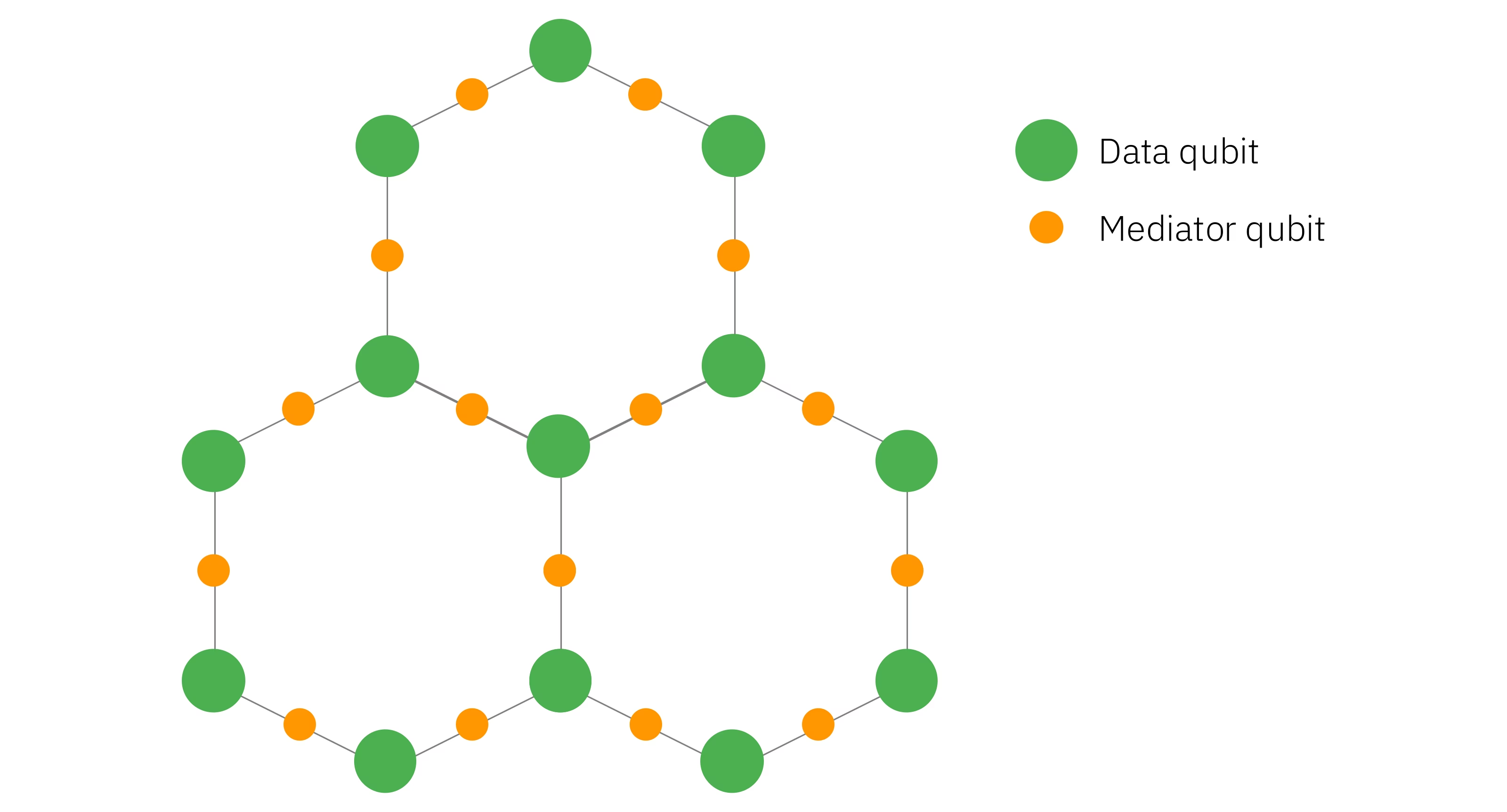 In this tutorial we will evaluate observables of a 22-site Ising model on a hexagonal lattice using a Heron QPU, which has a heavy-hexagonal qubit topology. Many demonstrations on Heron QPUs focus on systems defined on heavy-hexagonal lattices to match the system's connectivity; however, hexagonal models tend to be more interesting to study as they appear more commonly in nature and are more difficult to simulate classically due to their denser connectivity. Since the qubit topology of the QPU cannot directly support the connectivity of a hexagonal lattice, we must decide how to efficiently embed the hexagonal model onto the qubit topology. In this example we represent each site in the Ising model with a qubit lying on a vertex of the heavy-hex QPU lattice. We use the qubits on the edges (mediator qubits) to facilitate entanglement between the Ising qubits on the vertices. Additionally, the mediator qubits implement entanglement in such a way that they are always expected to return to the ground state . If a mediator qubit measures , it indicates that a logical error occurred during circuit execution; postselecting only samples with no detected errors on the mediator qubits yields a smaller distribution of logical samples that might have a higher fidelity than the raw, noisy distribution. Not only can we detect that an error occurred by measuring a mediator qubit, we can also determine exactly which logical errors that qubit is capable of detecting throughout the circuit. Removing the noise generators the mediator qubits' symmetry checks are capable of detecting from a noise model leaves a reduced noise model, which can be mitigated using techniques such as probabilistic error cancellation (PEC).
このノートブックの例では、上記のエラー検出技術とPECを組み合わせることで、いずれか一方の技術単独よりも効果的に量子ノイズに対処します。49量子ビットを使用して22量子ビットのイジングモデルを埋め込み、追加の27個のメディエーター量子ビットをエラー検出に使用します。対称性チェックをすり抜けるノイズを軽減するために、事後選択されたノイズチャネルに対してPECを実行します。エラー検出とPECの組み合わせに加えて、TREX読み出しエラー軽減や非マルコフエラーチェックなどの手法を使用して、量子ノイズの影響にさらに対処します。
ワークフローは次のとおりです。
- 22量子ビットの六角形イジングモデルに対する観測量の期待値を古典的にシミュレートする
- 量子回路を用いて49量子ビットのエラー検出六角形イジングモデルを実装し、QPUバックエンドへトランスパイルする
samplomaticを用いて回路内のエンタングリング層を指定する。これらのエンタングリング層に影響するノイズを学習し、軽減する。- 回路に非マルコフエラーチェックを追加する
- 回路に影響するゲートおよび読み出しノイズを学習する
- 対称性チェックで検出される項をノイズモデルから削除する
- エラー検出回路をサンプリングする。すべての対称性チェックおよび非マルコフエラーチェックに合格したサンプルのみを事後選択し、すべての期待値計算にTREX読み出し軽減を使用する
- エラー検出回路をサンプリングする
- PECを用いてエラー検出回路をサンプリングするが、対称性チェックに基づく事後選択は行わず、学習した完全なノイズチャネルを軽減する。
- PECを用いてエラー検出回路をサンプリングする。対称性チェックに基づいて事後選択を行い、チェックで検出できないノイズのみを軽減する。
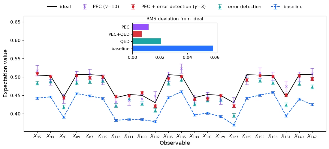
- 期待値を計算し、各戦略を比較する。QED+PECは、いずれかの手法単独よりも実験に影響するノイズを効果的にキャンセルし、PEC単独で必要なショット数よりもはるかに少ないショット数で収束した期待値を生成することを確認する。
要件
このチュートリアルを開始する前に、次のコマンドを実行して必要なパッケージをすべて取得してください。
%pip install networkx numpy "qiskit[visualization]" "qiskit-ibm-runtime[visualization]" samplomatic qiskit-mitigation matplotlib "qiskit-noise-learning @ git+https://github.com/Qiskit/qiskit-noise-learning.git@ieee-demo-2026"
以下の折りたたまれたセルは、このノートブック全体で使用される図のヘルパーを定義します。
クリックして図のヘルパーを表示
# Added by doQumentation — installs the packages this notebook needs if they are missing
import importlib.util

_needed = {"matplotlib": "matplotlib", "networkx": "networkx", "numpy": "numpy", "qiskit": "qiskit", "qiskit_ibm_runtime": "qiskit-ibm-runtime", "qiskit_mitigation": "qiskit-mitigation", "qiskit_noise_learning": "qiskit-noise-learning@git+https://github.com/Qiskit/qiskit-noise-learning.git@ieee-demo-2026", "samplomatic": "samplomatic"}
_missing = [pip for module, pip in _needed.items()
            if importlib.util.find_spec(module) is None]
# One at a time, so a package that fails to install does not block the others
for _pip in _missing:
    %pip install -q {_pip}
if not _missing:
    print("\u2713 All required packages are installed")
# Figure helpers for this notebook (collapsed): all plotting and styling lives here.
# The chip maps follow the style of Fig. 30 of arXiv:2607.25998.

from math import comb

import matplotlib.pyplot as plt
from matplotlib import cm
from matplotlib.colors import BoundaryNorm
from matplotlib.patches import Circle, Rectangle, Wedge

# one typography scheme for every figure in the notebook
plt.rcParams.update(
    {
        "font.size": 13,
        "axes.titlesize": 15,
        "axes.labelsize": 13,
        "xtick.labelsize": 11,
        "ytick.labelsize": 11,
        "legend.fontsize": 11,
    }
)

def x_labels(layout, n_data):
    """Per-observable tick labels carrying the physical qubit indices (site i = qubit i)."""
    return [f"$X_{{{layout[i]}}}$" for i in range(n_data)]

def plot_layout(backend, layout, n_data):
    """Chip cartoon of the embedding: data qubits green, check qubits orange."""
    from qiskit.visualization import plot_coupling_map

    return plot_coupling_map(
        num_qubits=backend.num_qubits,
        qubit_coordinates=None,
        coupling_map=list(backend.coupling_map.get_edges()),
        figsize=(9, 9),
        qubit_color=[
            "#4CAF50"
            if q in layout[:n_data]
            else "#FF9800"
            if q in layout[n_data:]
            else "#DDDDDD"
            for q in range(backend.num_qubits)
        ],
        qubit_size=220,
        line_width=2,
        font_size=90,
    )

def plot_exact(obs_exact, tick_labels, title):
    plt.figure(figsize=(12, 4))
    plt.plot(obs_exact, "o-")
    plt.title(title)
    plt.xticks(np.arange(len(obs_exact)), tick_labels)
    plt.xlabel("Observable")
    plt.ylabel(r"$\langle X \rangle$")
    plt.grid()

def draw_toy_circuit(
    generate_ed_ising, zz_coeff, x_coeff, include_checks=True
):
    """The boxing pipeline on a 3-plaquette-ring miniature (1 Trotter step) so the box
    structure is legible; every box carries the Twirl / InjectNoise annotations, and with
    ``include_checks`` the terminal xslow non-Markovian error check pattern is appended as in the
    production pipeline."""
    import networkx as nx
    from qiskit.circuit import ClassicalRegister
    from qiskit_mitigation.postselection import XSlowGate
    from samplomatic.transpiler import generate_boxing_pass_manager

    toy, _, _ = generate_ed_ising(nx.cycle_graph(3), 1, zz_coeff, x_coeff)
    toy.add_register(
        ClassicalRegister(3, "data"), ClassicalRegister(3, "check")
    )
    toy.barrier()
    toy.measure(range(3), range(3))
    toy.measure(range(3, 6), range(3, 6))
    toy_boxed = generate_boxing_pass_manager(
        enable_gates=True,
        enable_measures=True,
        inject_noise_targets="gates",
        inject_noise_strategy="individual_modification",
        inject_noise_site="after",
        twirling_strategy="active_circuit",
        measure_annotations="all",
    ).run(toy)
    if include_checks:
        toy_boxed.add_register(
            ClassicalRegister(3, "data_ps"), ClassicalRegister(3, "check_ps")
        )
        toy_boxed.barrier()
        for qb in range(6):
            toy_boxed.append(XSlowGate(), [qb])
        toy_boxed.measure(range(3), toy_boxed.cregs[2])
        toy_boxed.measure(range(3, 6), toy_boxed.cregs[3])
    return toy_boxed.draw("mpl", fold=-1, scale=0.6)

# --- chip-level noise maps ---------------------------------------------------------

BANDS = [1e-5, 2e-5, 3e-5, 4e-5, 6e-5, 1e-4, 2e-4, 3e-4, 4e-4, 6e-4, 1e-3]
CMAP = plt.get_cmap("YlOrBr")
NORM = BoundaryNorm(BANDS, CMAP.N, extend="both")

def _color(rate):
    return (
        "white"
        if rate < BANDS[0]
        else CMAP(NORM(min(rate, BANDS[-1] * 0.999)))
    )

def _layer_sparse(mit, weights):
    """Per-layer labelled terms from the saved run, box-local -> physical qubits."""
    phys = np.sort(mit["layout"])
    return [
        [
            (p, tuple(int(phys[q]) for q in qs if q >= 0), r)
            for p, qs, r in zip(
                mit[f"label_paulis_{i}"],
                mit[f"label_qubits_{i}"],
                w,
                strict=True,
            )
        ]
        for i, w in enumerate(weights)
    ]

def _aggregate(layers):
    """w1[qubit][P] and w2[(a,b)][PaPb]: rates summed over the 3 layers."""
    w1, w2 = {}, {}
    for terms in layers:
        for p, qs, r in terms:
            if len(qs) == 1:
                w1.setdefault(qs[0], dict.fromkeys("XYZ", 0.0))[p] += r
            else:
                (a, pa), (b, pb) = sorted(zip(qs, p, strict=True))
                w2.setdefault(
                    (a, b), {x + y: 0.0 for x in "XYZ" for y in "XYZ"}
                )[pa + pb] += r
    return w1, w2

def draw_noise_map(mit, backend, reduced=False):
    """Chip map of the learned model: X/Y/Z wheel per qubit, 3x3 two-qubit Pauli grid per
    coupler, log-banded colors, dashed outlines for unused hardware.

    With ``reduced=True``, keeps only the error terms the checks cannot see: detectability
    depends on circuit position, so each layer's 0/1 site scales are averaged over its uses.
    """
    from qiskit_ibm_runtime.visualization.embeddings import Embedding

    if reduced:
        scales = [
            mit["site_scales"][mit["site_layer"] == i].mean(axis=0)
            for i in range(3)
        ]
        weights = [mit[f"rates_{i}"] * scales[i] for i in range(3)]
        title = f"Reduced noise model ($\\gamma$ = {mit['gammas'][1]:.1f})"
    else:
        weights = [mit[f"rates_{i}"] for i in range(3)]
        title = f"Full noise model ($\\gamma$ = {mit['gammas'][0]:.0f})"
    w1, w2 = _aggregate(_layer_sparse(mit, weights))

    xy = np.array(
        [(c, -r) for r, c in Embedding.from_backend(backend).coordinates]
    )
    fig, ax = plt.subplots(figsize=(13, 7))
    for a, b in {tuple(sorted(e)) for e in backend.coupling_map.get_edges()}:
        if (
            (
                a,
                b,
            )
            in w2
        ):  # 3x3 Pauli grid laid along the bond (columns: qubit a, rows: qubit b)
            d = xy[b] - xy[a]
            u = d / np.hypot(*d)
            v = np.array([-u[1], u[0]])
            cl, cw = (np.hypot(*d) - 0.6) / 3, 0.17
            for i, Pa in enumerate("XYZ"):
                for j, Pb in enumerate("XYZ"):
                    ax.add_patch(
                        Rectangle(
                            xy[a] + u * (0.3 + i * cl) + v * ((j - 1.5) * cw),
                            cl,
                            cw,
                            angle=np.degrees(np.arctan2(u[1], u[0])),
                            facecolor=_color(w2[a, b][Pa + Pb]),
                            edgecolor="black",
                            lw=0.4,
                            zorder=2,
                        )
                    )
        else:
            ax.plot(
                *zip(xy[a], xy[b], strict=True),
                ls="--",
                lw=0.7,
                color="black",
                alpha=0.5,
                zorder=1,
            )
    for q, (xq, yq) in enumerate(xy):
        if q in w1:  # three-sector wheel: X top, Y lower left, Z lower right
            for P, t0 in (("X", 30), ("Y", 150), ("Z", 270)):
                ax.add_patch(
                    Wedge(
                        (xq, yq),
                        0.3,
                        t0,
                        t0 + 120,
                        facecolor=_color(w1[q][P]),
                        edgecolor="black",
                        lw=0.6,
                        zorder=3,
                    )
                )
            ax.annotate(
                str(q),
                (xq + 0.39, yq - 0.39),
                fontsize=9,
                color="gray",
                ha="left",
                va="top",
                zorder=4,
            )  # southeast, clear of the bond grids
        else:
            ax.add_patch(
                Circle(
                    (xq, yq),
                    0.24,
                    facecolor="none",
                    edgecolor="black",
                    ls="--",
                    lw=0.7,
                    alpha=0.5,
                    zorder=3,
                )
            )
    ux = xy[sorted(w1)]
    ax.set_xlim(ux[:, 0].min() - 2.2, ux[:, 0].max() + 2.2)
    ax.set_ylim(ux[:, 1].min() - 1.6, ux[:, 1].max() + 1.6)
    ax.set_aspect("equal")
    ax.axis("off")
    ax.set_title(title, fontsize=15)
    cb = fig.colorbar(
        cm.ScalarMappable(norm=NORM, cmap=CMAP),
        ax=ax,
        fraction=0.035,
        pad=0.02,
        extend="both",
        ticks=BANDS,
    )
    cb.set_label("coefficient (log bands; white < 1e-05)", fontsize=11)
    cb.ax.set_yticklabels(
        [f"{b:.0e}".replace("e-0", "e-") for b in BANDS], fontsize=10
    )
    _noise_map_legends(fig, ax)

def _noise_map_legends(fig, ax):
    """Weight-1 wheel and weight-2 grid keys, in a reserved band left of the lattice."""
    fig.subplots_adjust(left=0.17)
    axl = ax.inset_axes([-0.185, 0.70, 0.13, 0.24])
    for P, t0 in (("X", 30), ("Y", 150), ("Z", 270)):
        axl.add_patch(
            Wedge(
                (0.5, 0.45),
                0.38,
                t0,
                t0 + 120,
                facecolor="white",
                edgecolor="black",
                lw=0.8,
            )
        )
        axl.annotate(
            P,
            (
                0.5 + 0.2 * np.cos(np.radians(t0 + 60)),
                0.45 + 0.2 * np.sin(np.radians(t0 + 60)),
            ),
            ha="center",
            va="center",
            fontsize=9,
        )
    axl.set_title("weight-1", fontsize=10)
    axl.set_xlim(0, 1)
    axl.set_ylim(0, 1)
    axl.set_aspect("equal")
    axl.axis("off")
    axm = ax.inset_axes([-0.185, 0.32, 0.14, 0.30])
    for i, Pa in enumerate("XYZ"):
        for j, Pb in enumerate("XYZ"):
            axm.add_patch(
                Rectangle(
                    (i / 3, 1 - (j + 1) / 3),
                    1 / 3,
                    1 / 3,
                    facecolor="white",
                    edgecolor="black",
                    lw=0.6,
                )
            )
            axm.annotate(
                Pa + Pb,
                ((i + 0.5) / 3, 1 - (j + 0.5) / 3),
                ha="center",
                va="center",
                fontsize=7.5,
            )
        axm.annotate(Pa, ((i + 0.5) / 3, 1.08), ha="center", fontsize=8.5)
        axm.annotate(
            "XYZ"[i],
            (-0.13, 1 - (i + 0.5) / 3),
            ha="center",
            va="center",
            fontsize=8.5,
        )
    axm.annotate("qubit a", (0.5, 1.27), ha="center", fontsize=9)
    axm.annotate(
        "qubit b", (-0.33, 0.5), rotation=90, va="center", fontsize=9
    )
    axm.set_xlim(-0.35, 1.05)
    axm.set_ylim(-0.05, 1.35)
    axm.set_aspect("equal")
    axm.axis("off")

# --- run diagnostics ---------------------------------------------------------------

def plot_trex(trex_rescale, tick_labels):
    _fig, axt = plt.subplots(figsize=(12, 3))
    axt.stem(np.arange(len(trex_rescale)), (trex_rescale - 1) * 100)
    axt.set_xticks(np.arange(len(trex_rescale)), tick_labels)
    axt.set_xlabel("Observable")
    axt.set_ylabel("Readout correction (%)")
    axt.set_title("TREX rescale factors")
    plt.tight_layout()

def plot_postselection(mit):
    """Accepted shots per PEC randomization against a single binomial at the mean
    acceptance rate: agreement means acceptance is independent of the sampled circuit
    instance, the condition under which pooling accepted shots across randomizations
    is a consistent estimator."""
    _fig, ax = plt.subplots(figsize=(7.5, 3.8))
    counts = mit["acc_counts_post"]
    K, p = 64, counts.mean() / 64
    ks = np.arange(K + 1)
    pmf = np.array([comb(K, k) * p**k * (1 - p) ** (K - k) for k in ks])
    ax.hist(
        counts,
        bins=np.arange(-0.5, K + 1.5),
        density=True,
        alpha=0.6,
        color="#da1e28",
        label="measured",
    )
    ax.plot(ks, pmf, "k-", lw=1.5, label=f"Binomial(64, {p:.3f})")
    ax.set_xlim(-0.5, max(int(counts.max()) + 3, 20))
    ax.set_xlabel("Accepted shots per randomization")
    ax.set_ylabel("Probability")
    ax.legend()
    ax.grid(alpha=0.4)
    plt.tight_layout()

def plot_convergence(mit, obs_exact, n_data):
    """Running site-averaged estimate vs. randomizations for both PEC arms (the S5-consistent
    signed-ratio estimator, evaluated on growing prefixes of the sweep)."""

    def running(prefix):
        bits = np.squeeze(
            np.unpackbits(mit[f"data_{prefix}"], axis=-1)[..., :n_data]
            ^ mit[f"flips_{prefix}"]
        )
        mask = np.squeeze(mit[f"mask_{prefix}"])
        signs = 1 - 2 * (np.squeeze(mit[f"signs_{prefix}"]).sum(axis=-1) % 2)
        qv = (1 - 2 * bits.astype(int)) * mit["trex_rescale"]
        u = (
            (signs[:, None, None] * mask[..., None] * qv)
            .sum(axis=1)
            .mean(axis=1)
        )
        v = signs * mask.sum(axis=1)
        Rs = np.arange(500, len(u) + 1, 500)
        est, err = [], []
        for R in Rs:
            e = u[:R].sum() / v[:R].sum()
            est.append(e)
            err.append(
                np.sqrt(((u[:R] - e * v[:R]) ** 2).sum()) / abs(v[:R].sum())
            )
        return Rs, np.array(est), np.array(err)

    _fig, ax = plt.subplots(figsize=(12, 5))
    ideal_avg = float(np.mean(obs_exact))
    ax.axhline(ideal_avg, color="black", label="ideal")
    ax.fill_between(
        [-400, 24000],
        ideal_avg - 0.025,
        ideal_avg + 0.025,
        color="grey",
        alpha=0.22,
        label=r"$\pm 0.025$",
    )
    for prefix, label, color in (
        ("van", "vanilla PEC", "#8a3ffc"),
        ("post", "PEC + error detection", "#da1e28"),
    ):
        Rs, est, err = running(prefix)
        ax.errorbar(
            Rs,
            est,
            yerr=err,
            marker="o",
            linestyle="",
            markerfacecolor="none",
            color=color,
            alpha=0.85,
            capsize=3,
            label=label,
        )
    ax.set_xlim(-400, 24000)
    ax.set_ylim(ideal_avg - 0.08, ideal_avg + 0.08)
    ax.set_xlabel("# randomizations")
    ax.set_ylabel(r"Site-averaged $\langle X \rangle$")
    ax.legend(ncols=2)

def plot_final(
    obs_exact, baseline, ed, pec, post, gammas, tick_labels, title
):
    """Per-site <X> for every method, with an rms-deviation inset.
    baseline/ed/pec/post are (values, errors) pairs; gammas is (gamma, gamma_post)."""
    x = np.arange(len(obs_exact))
    _fig, ax = plt.subplots(figsize=(13, 5))
    h_ideal = ax.errorbar(
        x, obs_exact, fmt="-", capsize=4, label="ideal", color="black"
    )
    h_base = ax.errorbar(
        x,
        baseline[0],
        yerr=baseline[1],
        fmt=".--",
        capsize=4,
        label="baseline",
        color="#0f62fe",
    )
    h_ed = ax.errorbar(
        x,
        ed[0],
        yerr=ed[1],
        fmt="^",
        capsize=4,
        label="error detection",
        color="#009d9a",
        alpha=0.8,
    )
    h_pec = ax.errorbar(
        x,
        pec[0],
        yerr=pec[1],
        fmt="x",
        capsize=4,
        label=f"PEC ($\\gamma$={gammas[0]:.0f})",
        color="#8a3ffc",
        alpha=0.7,
    )
    h_post = ax.errorbar(
        x,
        post[0],
        yerr=post[1],
        fmt="d",
        capsize=4,
        label=f"PEC + error detection ($\\gamma$={gammas[1]:.0f})",
        color="#da1e28",
    )
    ax.set_xticks(x, tick_labels)
    ax.set_xlabel("Observable")
    ax.set_ylabel("Expectation value")
    # Set the y-axis range using the ideal, baseline, error detection, and PEC + error
    # detection curves, including error bars. Exclude PEC-only values when setting the
    # range so large fluctuations do not make the other curves difficult to distinguish.
    # PEC-only values may fall outside the visible range. Leave room above for the inset.
    series = [np.asarray(obs_exact)] + [
        np.asarray(v) + s * np.asarray(e)
        for v, e in (baseline, ed, post)
        for s in (-1, 1)
    ]
    lo, hi = min(a.min() for a in series), max(a.max() for a in series)
    span = max(hi - lo, 0.1)
    ax.set_ylim(lo - 0.1 * span, hi + 1.05 * span)
    # legend ordered to match the curves' vertical positions in the chart
    ax.legend(
        handles=[h_ideal, h_pec, h_post, h_ed, h_base],
        ncols=5,
        loc="lower center",
        bbox_to_anchor=(0.5, 1.02),
        frameon=False,
    )
    ax.set_title(title, pad=44)

    # inset: rows bottom-to-top so it reads top-to-bottom: PEC, PEC+ED, ED, baseline
    axi = ax.inset_axes([0.36, 0.68, 0.28, 0.26])
    methods = [
        ("baseline", baseline[0], "#0f62fe"),
        ("QED", ed[0], "#009d9a"),
        ("PEC+QED", post[0], "#da1e28"),
        ("PEC", pec[0], "#8a3ffc"),
    ]
    for k, (_nm, vals, color) in enumerate(methods):
        axi.barh(
            k,
            np.sqrt(np.mean((vals - np.array(obs_exact)) ** 2)),
            color=color,
            alpha=0.9,
        )
    axi.set_yticks(range(4), [m[0] for m in methods], fontsize=10)
    axi.set_title("RMS deviation from ideal", fontsize=11)
    axi.tick_params(labelsize=10)
    axi.patch.set_alpha(1.0)
    axi.set_zorder(5)
22量子ビットの六角形イジングモデルの各サイトにおける を古典的にシミュレートする
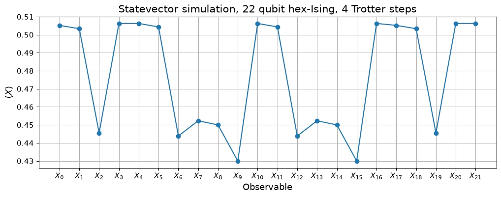
まず、Qiskitの Statevector クラスを使用して、実験の正確な目標値をシミュレートします。私たちが解いている22量子ビットの問題は古典的に扱いやすいものですが、Qiskitのステートベクトルシミュレーターはこれよりもかなり大きなデモにはスケールしません。50量子ビット程度を超えてスケールアップするには、パウリ伝播のような近似的なシミュレーション手法を使用する必要があります。この49量子ビットの実験により、理想的な期待値へのアクセスを維持しながら、より大きなスケールでエラー検出とエラー軽減を組み合わせることを調査できます。
import warnings

import networkx as nx
import numpy as np
from qiskit.circuit import QuantumCircuit
from qiskit.quantum_info import Pauli, Statevector

# Silence two harmless upstream warnings (a Samplomatic default-change notice and a
# numpy datetime timezone notice from the noise-learning circuit generator)
warnings.filterwarnings(
    "ignore", message="The default of the 'inject_noise_site'"
)
warnings.filterwarnings(
    "ignore", message="no explicit representation of timezones"
)

# Hexagonal lattice
data_graph = nx.convert_node_labels_to_integers(
    nx.hexagonal_lattice_graph(2, 3)
)

# Number of Trotter steps and rotation angles
depth = 4
zz_coeff = -np.pi / 4
x_coeff = 3 * np.pi / 8
n_data = data_graph.order()
n_checks = data_graph.size()
n_qubits = n_data + n_checks

qc_data = QuantumCircuit(n_data)
qc_data.h(range(n_data))
for _ in range(depth):
    for edge in data_graph.edges:
        qc_data.rzz(zz_coeff, *edge)
    qc_data.rx(x_coeff, range(n_data))
psi_exact = Statevector(qc_data)

# X on site i = qubit i
observables = ["I" * (n_data - 1 - i) + "X" + "I" * i for i in range(n_data)]
obs_exact = [psi_exact.expectation_value(Pauli(o)).real for o in observables]

plot_exact(
    obs_exact,
    x_labels(range(n_data), n_data),
    f"Statevector simulation, {n_data} qubit hex-Ising, {depth} Trotter steps",
)
量子回路を用いて49量子ビットのエラー検出六角形イジングモデルを実装し、QPUバックエンドへトランスパイルする
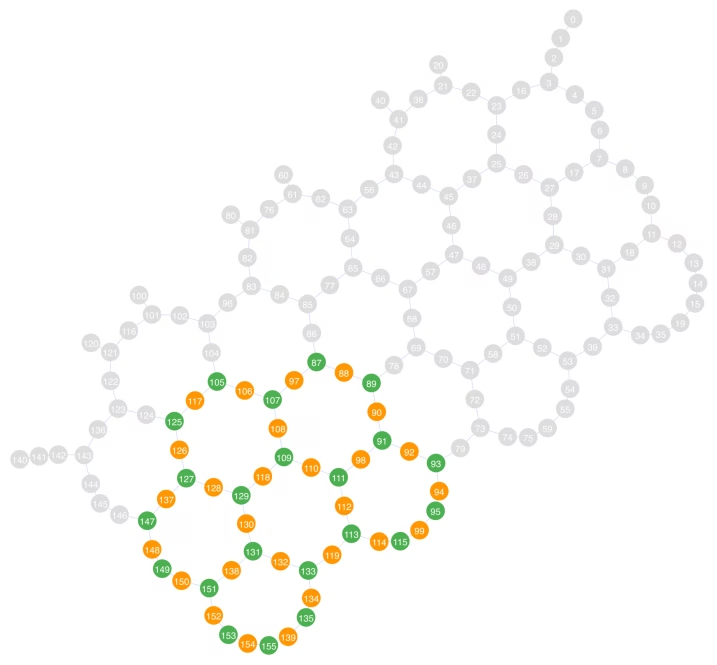
この回路は、六角形格子上の22量子ビットの横磁場イジングハミルトニアンの4回のトロッター・ステップをシミュレートします。22個のデータ量子ビットは、Heron r3 QPUである ibm_boston の49量子ビットのヘビーヘックス部分グラフに埋め込まれます。27個の補助量子ビットは、イジング量子ビット間のエンタングルメントを媒介することと、回路実行中の論理エラーを検出することという2つの目的で使用されます。回路のエンタングリング層は、メディエーター量子ビットが最終測定前に基底状態 に戻るように実装されています。1つ以上のメディエーター量子ビットが を測定した場合、そのサンプルは論理エラーによって破損したことを示します。これらのサンプルを破棄することで、サンプリングされた分布の忠実度を向上させることができます。
下のグラフでは、緑色の量子ビットが22個のイジング量子ビットを表し、オレンジ色の量子ビットが27個のメディエーター量子ビットを表します。
from qiskit.circuit import ClassicalRegister
from qiskit.transpiler import generate_preset_pass_manager
from qiskit_ibm_runtime import QiskitRuntimeService

backend_name = "ibm_boston"

def generate_ed_ising(graph, depth, zz_coeff, x_coeff):
    """Build the mediated error-detecting Ising circuit for data-qubit `graph`; returns (circuit, CZ layers, hardware graph)."""
    hw_graph = nx.Graph()
    for i, (a, b) in enumerate(graph.edges()):
        hw_graph.add_edges_from(
            [(a, i + graph.order()), (b, i + graph.order())]
        )
    coloring = nx.coloring.greedy_color(
        nx.line_graph(hw_graph), strategy="DSATUR"
    )
    layers_coupling = [
        [e for e, c in coloring.items() if c == i]
        for i in set(coloring.values())
    ]
    circuit = QuantumCircuit(hw_graph.order())
    circuit.h(range(hw_graph.order()))
    for _ in range(depth):
        for angle, qubits in (
            (zz_coeff, range(graph.order(), hw_graph.order())),
            (x_coeff, range(graph.order())),
        ):
            circuit.barrier()
            for layer in layers_coupling:
                for edge in layer:
                    circuit.cz(*edge)
            circuit.barrier()
            circuit.rx(angle, qubits)
    circuit.barrier()
    circuit.h(range(graph.order(), hw_graph.order()))
    return circuit, layers_coupling, hw_graph

service = QiskitRuntimeService()
backend = service.backend(backend_name)

circuit, layers_coupling, hw_graph = generate_ed_ising(
    data_graph, depth, zz_coeff, x_coeff
)

circ_meas = circuit.copy()
data_reg, check_reg = (
    ClassicalRegister(n_data, "data"),
    ClassicalRegister(n_checks, "check"),
)
circ_meas.add_register(data_reg, check_reg)
circ_meas.barrier()
circ_meas.measure(range(n_data), data_reg)
circ_meas.measure(range(n_data, n_qubits), check_reg)

# Physical qubits hosting the 22 Ising sites on ibm_boston, one heavy-hex row per lattice chain;
# the mediator for each edge is the physical qubit sitting between its two data qubits
data_layout = [
    *[95, 93, 91, 89, 87],
    *[115, 113, 111, 109, 107, 105],
    *[135, 133, 131, 129, 127, 125],
    *[155, 153, 151, 149, 147],
]
coupling_graph = nx.Graph(list(backend.coupling_map.get_edges()))
layout = data_layout + [
    next(
        iter(
            nx.common_neighbors(
                coupling_graph, data_layout[a], data_layout[b]
            )
        )
    )
    for a, b in data_graph.edges()
]

circ_trans = generate_preset_pass_manager(
    backend=backend, optimization_level=1, initial_layout=layout
).run(circ_meas)

plot_layout(backend, layout, n_data)
samplomatic を用いて回路内のエンタングリング層を指定する。
Samplomaticの generate_boxing_pass_manager パスは、回路のエンタングリング層をパウリツイリングとPECノイズ注入のためのアノテーション付きボックスにグループ化します。得られたテンプレート回路とサンプレックス(テンプレート回路上のツイリングとノイズ注入を指定するパラメトリック分布)は、すべてのノイズ学習およびサンプリングのQPU実験を定義・実行するために使用されます。測定ボックスには ChangeBasis アノテーションも付与されており、データ量子ビットをX基底で測定する回転は、回路に焼き込まれるのではなく、サンプリング時にサンプレックスへの入力として供給されます。
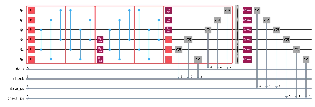
以下では、同じボクシングパスをエラー検出イジング回路の小さなバージョンに適用し、ボックス化された回路の構造を可視化できるようにします。
from samplomatic.builders import build
from samplomatic.transpiler import generate_boxing_pass_manager
from samplomatic.utils import find_unique_box_instructions

boxed = generate_boxing_pass_manager(
    enable_gates=True,
    enable_measures=True,
    inject_noise_targets="gates",
    inject_noise_strategy="individual_modification",
    inject_noise_site="after",
    twirling_strategy="active_circuit",
    measure_annotations="all",
).run(circ_trans)
template, samplex = build(boxed)
unique_instructions = find_unique_box_instructions(
    boxed, normalize_annotations=None, undress_boxes=True
)

# Measure X on the data qubits and Z on the mediators
basis_key = next(
    s.name
    for s in samplex.inputs().get_specs()
    if s.name.startswith("basis_changes.")
)
meas_basis = np.array(
    [2 if q in set(layout[:n_data]) else 1 for q in sorted(layout)],
    dtype=np.uint8,
)

draw_toy_circuit(generate_ed_ising, zz_coeff, x_coeff, include_checks=False)

回路に非マルコフエラーチェックを追加する
次に、学習プロトコルでモデル化されていないノイズから保護するために、回路に非マルコフエラーチェックを追加します。これらのチェックは、長いパルスのビットフリップを実装し、量子ビットがある古典状態から別の古典状態へ正しく移行したことを確認することで機能します。エッジ上の両方の量子ビットがチェックに失敗した場合、そのサンプルは破棄されます。非マルコフエラーチェックは回路の先頭または末尾(あるいは両方)で使用できますが、ここでは末尾でのみ使用します。また、回路に隣接する未使用の「観客(スペクテーター)」量子ビットにもチェックを配置し、これらのチェックが検出するよう設計されたノイズに対するカバレッジを高めます。
対称性チェックと同様に、これも一種の事後選択であることに留意してください。そのため、これらの手法を組み合わせる際には、事後選択率の低下を考慮する必要があります。具体的には、、 とすると、1つの論理サンプルを復元するにはおよそ 個のノイズを含むサンプルが必要です。
from qiskit.transpiler import PassManager
from qiskit_mitigation.postselection import PostSelector
from qiskit_mitigation.postselection.passes import (
    AddPostCircuitNonMarkovianErrorChecks,
    AddSpectatorPostCircuitNonMarkovianErrorChecks,
)

add_checks = PassManager(
    [
        AddPostCircuitNonMarkovianErrorChecks(x_pulse_type="xslow"),
        AddSpectatorPostCircuitNonMarkovianErrorChecks(
            backend.coupling_map, x_pulse_type="xslow"
        ),
    ]
)
template_checked = add_checks.run(template)
selector = PostSelector.from_circuit(template_checked, backend.coupling_map)

draw_toy_circuit(generate_ed_ising, zz_coeff, x_coeff, include_checks=True)
49量子ビットのチェック付きイジング回路のゲートおよび読み出しノイズを学習する
ノイズを軽減するには、ノイズがエンタングリングゲートにどのように影響しているかをモデル化する必要があります。ここでは、qiskit-noise-learningを使用して、回路の3つの固有のエンタングリング層それぞれについてパウリ・リンドブラッドノイズモデルを学習します。後で、対称性チェックによって検出可能なエラー生成子をこのノイズモデルから削除し、残りのノイズチャネルのみをPECで軽減します。以下のマップは、QPU上で学習された3つの層を示しています。各量子ビットはその重み1のX/Y/Zレートのホイールであり、各カプラーはそのペアの重み2のパウリレートの3×3グリッドです。 の値が であることは、サンプリングオーバーヘッドが であることを意味します。
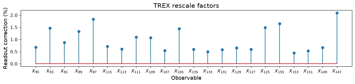
読み出し(TREX)補正は、ノイズ学習フィットのSPAMパスから直接得られます。QPUノイズマップの下にあるステムプロットは、観測量ごとのTREX再スケール係数を示しています。
from qiskit.quantum_info import PauliLindbladMap, QubitSparsePauli
from qiskit_ibm_runtime import Executor, Session
from qiskit_ibm_runtime.quantum_program import QuantumProgram
from qiskit_mitigation.trex import TREX
from qiskit_noise_learning.analysis import (
    ComputeObservables,
    CurveFitObservables,
    FlipPostSelect,
    LeastSquaresSolve,
)
from qiskit_noise_learning.circuit_generator import ExecutorCircuitGenerator
from qiskit_noise_learning.experiment_builder import (
    BindFragmentDepths,
    CompleteSequences,
    EvenDepthVanillaPaths,
    Experiment,
    GenerateInstructionSequences,
    IdentifyRelations,
    MergeInstructionSequences,
    SPAMPaths,
    VanillaInstructionSequences,
)
from qiskit_noise_learning.gate_sets import QiskitGateSet
from qiskit_noise_learning.models import PauliLindbladModel
from qiskit_noise_learning.models.utils import split_pauli_lindblad_model
from samplomatic.annotations import InjectNoise
from samplomatic.utils import get_annotation

gate_set = QiskitGateSet(
    target=backend.target,
    qubit_subset=sorted(
        {
            boxed.find_bit(q).index
            for i in unique_instructions
            for q in i.qubits
        }
    ),
)
ref_to_qubits = {}
for inst in unique_instructions:
    if ann := get_annotation(inst.operation, InjectNoise):
        gate_set.add_box_as_gate(inst, name=ann.ref)
        ref_to_qubits[ann.ref] = sorted(
            boxed.find_bit(q).index for q in inst.qubits
        )

fidelity_model = PauliLindbladModel.k_local(
    gate_set, gate_k={**{r: 2 for r in ref_to_qubits}, "M": 1, "P": 1}
)
experiment = (
    EvenDepthVanillaPaths()
    + VanillaInstructionSequences()
    + IdentifyRelations()
    + SPAMPaths()
    + GenerateInstructionSequences()
    + MergeInstructionSequences()
    + CompleteSequences()
    + BindFragmentDepths([2, 4, 8, 12])
).run(Experiment(fidelity_model=fidelity_model, shots=384, randomizations=64))

circuit_generator = ExecutorCircuitGenerator(
    gate_set, pass_manager=add_checks
)
program_learn, data_mapper = circuit_generator.generate(experiment)

session = Session(backend)
executor_options = {"environment": {"job_tags": ["TUT_PECLNM"]}}
fit = circuit_generator.collect(
    Executor(session, options=executor_options).run(program_learn).result(),
    data_mapper,
)
fit = (
    FlipPostSelect()
    + ComputeObservables()
    + CurveFitObservables()
    + LeastSquaresSolve()
).run(fit)
print(
    "learning shots removed by checks:",
    f"{float(fit.raw_data.datatree['0']['data_mask'].mean()):.4f}",
)

# TREX factors from the fit's SPAM paths: the fit only identifies the product of
# state-prep and measurement error, so hand TREX the composition of the two maps
spam = fidelity_model.to_pauli_lindblad_maps(
    fit.model_data, include_spam=True
)
spam_map = spam["P"].compose(spam["M"])
z_terms = [
    QubitSparsePauli(("Z", [layout[i]]), num_qubits=backend.num_qubits)
    for i in range(n_data)
]
trex_rescale = np.array(
    [TREX.calculate_trex_factor(spam_map, z) for z in z_terms]
)

# learned maps come back in backend qubit indexing; samplex wants box-local order
plm = split_pauli_lindblad_model(fit.model).model
noise_maps = {}
for ref, m in plm.to_pauli_lindblad_maps(fit.model_data).items():
    box = ref_to_qubits[ref]
    noise_maps[ref] = PauliLindbladMap.from_sparse_list(
        [
            (p, tuple(box.index(q) for q in qs), r)
            for p, qs, r in m.to_sparse_list()
        ],
        num_qubits=len(box),
    )
# Full-PEC cost: each learned layer acts twice per Trotter step (compute + uncompute)
gamma = float(
    np.exp(2 * depth * sum(2 * sum(m.rates) for m in noise_maps.values()))
)

# Collect the learned model in the form the figure helpers expect
mit = dict(
    **{
        f"rates_{i}": np.asarray(m.rates)
        for i, m in enumerate(noise_maps.values())
    },
    **{
        f"label_paulis_{i}": np.array([p for p, _, _ in m.to_sparse_list()])
        for i, m in enumerate(noise_maps.values())
    },
    **{
        f"label_qubits_{i}": np.array(
            [
                list(qs) + [-1] * (2 - len(qs))
                for _, qs, _ in m.to_sparse_list()
            ]
        )
        for i, m in enumerate(noise_maps.values())
    },
    layout=np.array(layout),
    trex_rescale=trex_rescale,
    gammas=np.array([gamma, np.nan]),
)
draw_noise_map(mit, backend)
plot_trex(mit["trex_rescale"], x_labels(layout, n_data))
learning shots removed by checks: 0.2393
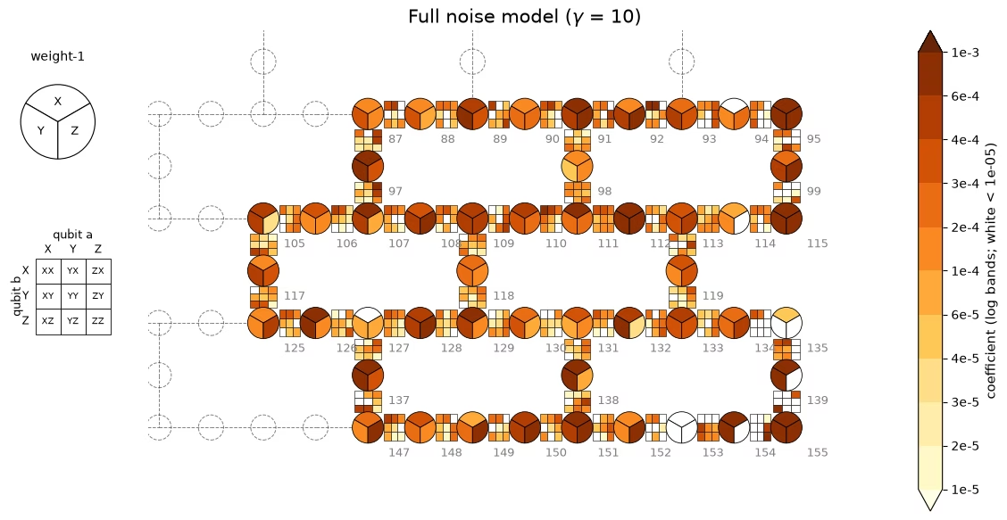
対称性チェックで検出可能な項をノイズモデルから削除する
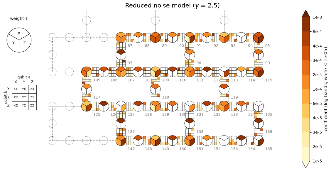
各対称性チェックは、ノイズモデル内のエラー生成子のあるサブセットを検出できるため、それらのエラーを軽減する必要はありません。ここでは、qiskit_mitigation の create_postselected_noise_mask 関数を使用して、検出可能なノイズ生成子のマスクを作成します。このマスクは、PECを実行する前に、検出可能な項をノイズモデルから削除するために使用されます。上記のノイズモデルマップに示されているように、削除後のノイズモデルに対してPECを実行すると、完全なノイズモデルに対してPECを実行するのに必要なサンプリングコストのごく一部で、収束した期待値を得ることができます。
以下のマップは、上記の学習済みモデルと同じカラースケールで描かれており、チェックで検出できないエラー生成子のみを残しています。多数のエラー生成子がモデルから削除され、サンプリングオーバーヘッドが大幅に低下していることが分かります。削除後のノイズモデルに対してPECを実行するためのサンプリングオーバーヘッドは であり、完全なノイズチャネルを軽減するために必要なオーバーヘッドからおよそ16倍の削減となります。
from qiskit.quantum_info import Pauli
from qiskit_mitigation.noise import create_postselected_noise_mask

SHOTS_PER_RAND = 64  # shots per PEC randomization
N_RAND = 23_054  # PEC randomizations per experiment
MAX_PAIR_RATE = 0.02  # Max value of any coupler's summed two-qubit error rate

# The detectors are virtual Pauli-Z's representing the measurements on the mediator qubits
# We can find the set of detectable noise generators in the model for each detector by conjugating
# it backward through the circuit and calculating what generators it anti-commutes with.
detectors = [
    Pauli("I" * (boxed.num_qubits - 1 - q) + "Z" + "I" * q)
    for q in layout[n_data:]
]
# Detectable generators are handled by postselection; prune them from the model for PEC
local_scales, gamma2_post = create_postselected_noise_mask(
    boxed, noise_maps, detectors
)
gamma_post = gamma2_post**0.5
print(f"gamma PEC {gamma:.2f} | gamma QED+PEC {gamma_post:.2f}")

# Kill the job if any coupler's summed rate exceeds MAX_PAIR_RATE
pair_lam = {}
for m in noise_maps.values():
    for _, qs, r in m.to_sparse_list():
        if len(qs) == 2:
            pair_lam[tuple(sorted(qs))] = (
                pair_lam.get(tuple(sorted(qs)), 0.0) + r
            )
assert (
    max(pair_lam.values()) < MAX_PAIR_RATE
), f"kill: degraded coupler {max(pair_lam, key=pair_lam.get)}"

# Detectability depends on circuit position, so record each site's 0/1 scales by layer
site_ref = {
    a.modifier_ref: a.ref
    for inst in boxed.data
    if inst.operation.name == "box"
    and (a := get_annotation(inst.operation, InjectNoise))
    and a.ref
}
sites = sorted(local_scales, key=lambda s: int(s[1:]))
mit["site_scales"] = np.stack([local_scales[s] for s in sites])
mit["site_layer"] = np.array(
    [list(noise_maps).index(site_ref[s]) for s in sites]
)
mit["gammas"] = np.array([gamma, gamma_post])
draw_noise_map(mit, backend, reduced=True)
gamma PEC 10.08 | gamma QED+PEC 2.52
エラー検出回路をサンプリングする
ここでは、49量子ビットのエラー検出イジング回路をサンプリングします。パウリツイリングと非マルコフエラーチェックを有効にしますが、PECサンプリングは行いません。これらのサンプルを使用して、ベースラインの期待値と、エラー検出のみを適用した期待値を計算します。
# Baseline = the ED+PEC template itself at noise scale 0, i.e. twirling only
program_tw = QuantumProgram(shots=100)
program_tw.append_samplex_item(
    template_checked,
    samplex=samplex,
    shape=(1000, 1),
    samplex_arguments={
        "pauli_lindblad_maps": dict(noise_maps),
        basis_key: meas_basis,
        **{f"noise_scales.{k}": 0.0 for k in local_scales},
    },
)
job_tw = Executor(session, options=executor_options).run(program_tw)
PECを用いてエラー検出回路をサンプリングする
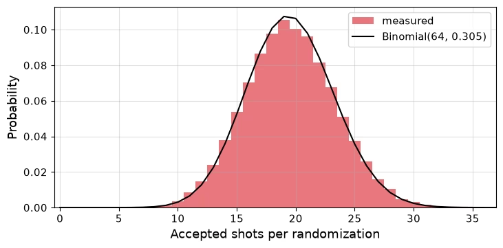
ここで再度サンプリングを行い、対称性チェックで検出できないノイズを軽減するためのPECランダム化を含めます。これらのサンプルは、エラー検出とPECを組み合わせて期待値を計算するために使用されます。以下では、PECランダム化ごとの受理ショット数を、平均受理率における二項分布と比較してプロットします。QED+PECは、すべてのメディエーター量子ビットの測定と交換可能な検出不可能なパウリのみを注入するため、受理率がサンプリングされた回路インスタンスと無相関であることが分かります。
def launch(session, template, samplex, samplex_args, n_rand, shots_per_rand):
    """Sample `n_rand` randomizations of `template` on `session` in <=100k-randomization jobs; returns the jobs."""
    jobs = []
    for start in range(0, n_rand, 100_000):
        program = QuantumProgram(shots=shots_per_rand)
        program.append_samplex_item(
            template,
            samplex=samplex,
            samplex_arguments=samplex_args,
            shape=(min(100_000, n_rand - start), 1),
        )
        jobs.append(Executor(session, options=executor_options).run(program))
    return jobs

# Reduced PEC
args_post = {
    "pauli_lindblad_maps": dict(noise_maps),
    basis_key: meas_basis,
    **{f"noise_scales.{k}": -1.0 for k in local_scales},
    **{f"local_scales.{k}": v for k, v in local_scales.items()},
}
# PEC on the full noise model
args_van = {
    "pauli_lindblad_maps": dict(noise_maps),
    basis_key: meas_basis,
    **{f"noise_scales.{k}": -1.0 for k in local_scales},
}

# Run sampling jobs
jobs = launch(
    session, template_checked, samplex, args_post, N_RAND, SHOTS_PER_RAND
)
jobs_van = launch(
    session, template_checked, samplex, args_van, N_RAND, SHOTS_PER_RAND
)
outs = [j.result()[0] for j in jobs]
outs_van = [j.result()[0] for j in jobs_van]
(out_tw,) = job_tw.result()
session.close()
サンプルを収集し、PECランダム化がメディエーター量子ビットの測定と交換可能であり、事後選択の統計に影響を与えないことを確認します。
def bitflip_mask(out, selector):
    """Per-shot True/False for job result `out`: shot passes `selector`'s non-Markovian error checks."""
    regs = {
        k: np.asarray(out[k])
        for k in out
        if not k.startswith(("measurement_flips", "pauli_signs"))
    }
    return selector.compute_mask(regs, "edge", mode="post")

def symmetry_mask(out):
    """Per-shot True/False for job result `out`: every twirl-corrected symmetry check reads 0."""
    return ~(
        np.asarray(out["check"]) ^ np.asarray(out["measurement_flips.check"])
    ).any(axis=-1)

def keep_mask(out, selector):
    """Per-shot True/False for job result `out`: shot passes both check types."""
    return symmetry_mask(out) & bitflip_mask(out, selector)

def fracs(out_list, selector):
    """Fractions of shots across the job results in `out_list` passing [no, non-Markovian error, symmetry, both] checks."""
    bf = np.concatenate([bitflip_mask(o, selector) for o in out_list])
    sy = np.concatenate([symmetry_mask(o) for o in out_list])
    return [1.0, bf.mean(), sy.mean(), (bf & sy).mean()]

mask_post = np.concatenate([keep_mask(o, selector) for o in outs])

# Collect the sampled data alongside the learned model, in the form the figure helpers expect
mit.update(
    ps_fracs=np.array(
        [
            fracs([out_tw], selector),
            fracs(outs_van, selector),
            fracs(outs, selector),
        ]
    ),
    acc_counts_post=np.squeeze(mask_post).sum(axis=-1),
    data_tw=np.asarray(out_tw["data"]),
    flips_tw=np.asarray(out_tw["measurement_flips.data"]),
    mask_tw=keep_mask(out_tw, selector),
    data_post=np.packbits(
        np.concatenate([np.asarray(o["data"]) for o in outs]), axis=-1
    ),
    flips_post=np.concatenate(
        [np.asarray(o["measurement_flips.data"]) for o in outs]
    ),
    signs_post=np.concatenate([np.asarray(o["pauli_signs"]) for o in outs]),
    mask_post=mask_post,
    data_van=np.packbits(
        np.concatenate([np.asarray(o["data"]) for o in outs_van]), axis=-1
    ),
    flips_van=np.concatenate(
        [np.asarray(o["measurement_flips.data"]) for o in outs_van]
    ),
    signs_van=np.concatenate(
        [np.asarray(o["pauli_signs"]) for o in outs_van]
    ),
    mask_van=np.concatenate([bitflip_mask(o, selector) for o in outs_van]),
)

# Plot the PEC bias check
plot_postselection(mit)
期待値を計算し、各戦略を比較する
最後に、qiskit-mitigation の executor_expectation_values ヘルパー関数を使用してすべての期待値を計算します。この関数は、測定フリップ、事後選択マスク、TREX再スケール係数、および準確率符号を適用してくれます。
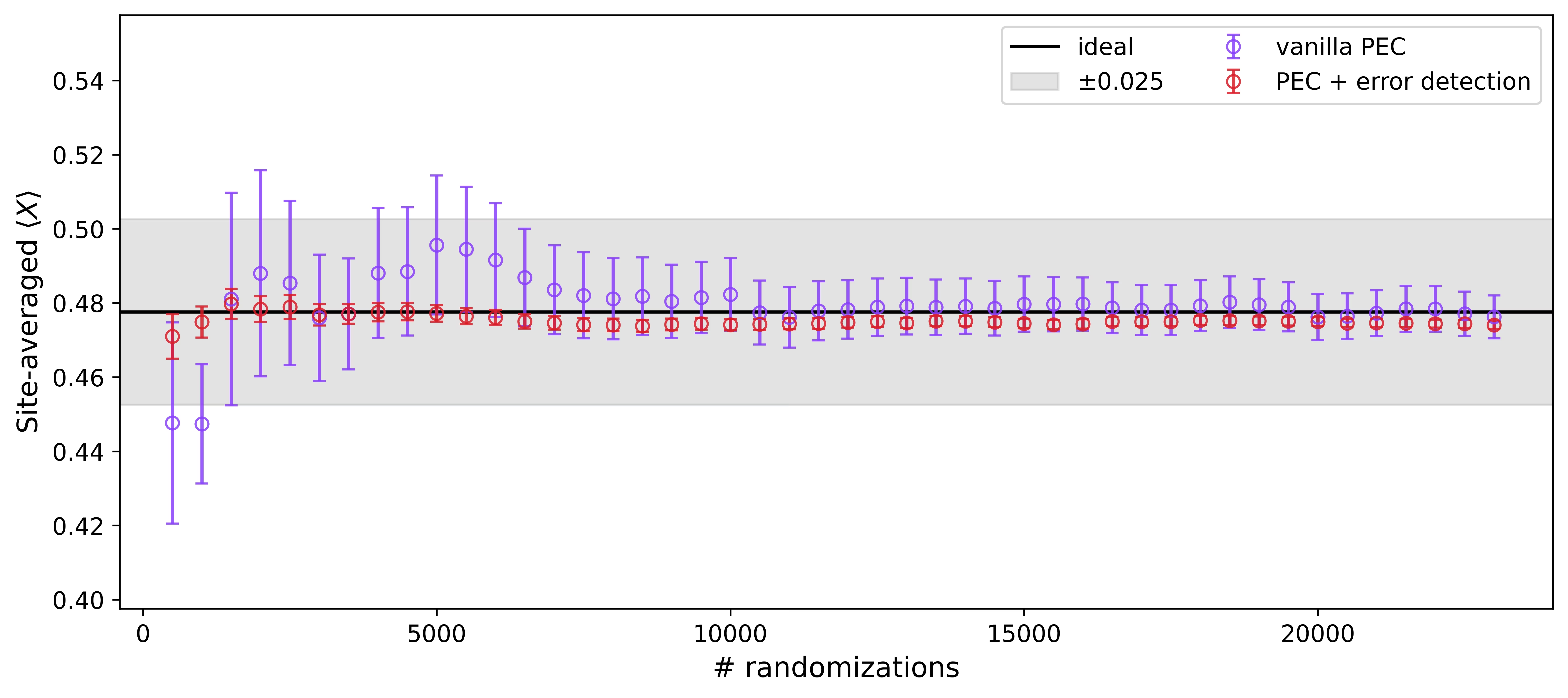
上のグラフ: 両方のPECバリアントが収束することが分かりますが、QED+PECはより少ないランダム化回数で、より狭い誤差範囲で の帯域に到達します。QED+PECの計算における残留バイアスは0.01未満であり、ノイズモデルの不一致、時間経過による量子ビットのドリフト、モデル化されていないノイズ源の影響の組み合わせに起因すると考えられます。
下のグラフ: 両方のPECバリアントについて、ランダム化ごとに同じショット数を使用してランダム化を積み重ねた際の、サイト平均 の逐次推定値です。PEC+エラー検出は数千回のランダム化以内に帯域内に収まりますが、完全なサンプリングオーバーヘッドを払うPEC単独では、収束するためにはるかに多くのランダム化が必要です。
from qiskit.quantum_info import SparsePauliOp
from qiskit_mitigation.utils import executor_expectation_values

gamma, gamma_post = mit["gammas"]
basis_map = {Pauli("X" * n_data): [SparsePauliOp(o) for o in observables]}
rescale = dict(zip(observables, mit["trex_rescale"], strict=True))

def evs(bits, basis_map, **kwargs):
    """Per-site (means, standard errors) from boolean shot data `bits` of shape (rands, 1, shots, n_data)."""
    out = executor_expectation_values(
        bits, basis_map, None, avg_axis=(0, 1), **kwargs
    )
    return np.array([m for m, _ in out]).ravel(), np.sqrt(
        [v for _, v in out]
    ).ravel()

def unpack(mit, prefix, n_data):
    """Restore `mit[f"data_\{prefix\}"]` from packed bytes to booleans of shape (rands, 1, shots, n_data)."""
    return np.unpackbits(mit[f"data_{prefix}"], axis=-1)[..., :n_data].astype(
        bool
    )

unmit_tw, unmit_tw_err = evs(
    mit["data_tw"], basis_map, measurement_flips=mit["flips_tw"]
)
ed_tw, ed_tw_err = evs(
    mit["data_tw"],
    basis_map,
    measurement_flips=mit["flips_tw"],
    postselect_mask=mit["mask_tw"],
    rescale_factors=rescale,
)
post, post_err = evs(
    unpack(mit, "post", n_data),
    basis_map,
    measurement_flips=mit["flips_post"],
    pauli_signs=mit["signs_post"],
    postselect_mask=mit["mask_post"],
    rescale_factors=rescale,
)
pec, pec_err = evs(
    unpack(mit, "van", n_data),
    basis_map,
    measurement_flips=mit["flips_van"],
    pauli_signs=mit["signs_van"],
    postselect_mask=mit["mask_van"],
    rescale_factors=rescale,
)

# effective ED+PEC overhead measured from the data: accepted shots per signed accepted shot
signs_post = 1 - 2 * (np.squeeze(mit["signs_post"]).sum(axis=-1) % 2)
gamma_eff = (
    mit["mask_post"].sum()
    / (signs_post * np.squeeze(mit["mask_post"]).sum(axis=-1)).sum()
)

print(
    f"gamma PEC {gamma:.2f} | gamma QED+PEC {gamma_post:.2f} (model) / {gamma_eff:.2f} (data) | "
    f"QED survival {mit['mask_tw'].mean():.3f} | QED+PEC survival {mit['mask_post'].mean():.3f} | "
    f"mean QED+PEC err {post_err.mean():.4f}"
)
plot_final(
    obs_exact,
    (unmit_tw, unmit_tw_err),
    (ed_tw, ed_tw_err),
    (pec, pec_err),
    (post, post_err),
    (gamma, gamma_post),
    x_labels(layout, n_data),
    "",
)
gamma PEC 10.08 | gamma QED+PEC 2.52 (model) / 2.51 (data) | QED survival 0.304 | QED+PEC survival 0.305 | mean QED+PEC err 0.0037
plot_convergence(mit, obs_exact, n_data)