部分空間の次元の上限設定
このウォークスルーでは、自己無撞着な配置回復手法における部分空間の次元の影響を示します。
事前には、目標の精度を得るために正しい部分空間の次元がどれであるかはわかりません。しかし、部分空間の次元を大きくすると、この手法の精度が向上することはわかっています。そのため、部分空間の次元の関数として予測の精度を調べることができます。 分子とその特性を指定します。
# Added by doQumentation — installs the packages this notebook needs if they are missing
import importlib.util

_needed = {"matplotlib": "matplotlib", "numpy": "numpy", "pyscf": "pyscf", "qiskit_addon_sqd": "qiskit-addon-sqd"}
_missing = [pip for module, pip in _needed.items()
            if importlib.util.find_spec(module) is None]
# One at a time, so a package that fails to install does not block the others
for _pip in _missing:
    %pip install -q {_pip}
if not _missing:
    print("\u2713 All required packages are installed")
import warnings

import pyscf
import pyscf.cc
import pyscf.mcscf

warnings.filterwarnings("ignore")

# Specify molecule properties
open_shell = False
spin_sq = 0

# Build N2 molecule
mol = pyscf.gto.Mole()
mol.build(
    atom=[["N", (0, 0, 0)], ["N", (1.0, 0, 0)]],
    basis="6-31g",
    symmetry="Dooh",
)

# Define active space
n_frozen = 2
active_space = range(n_frozen, mol.nao_nr())

# Get molecular integrals
scf = pyscf.scf.RHF(mol).run()
num_orbitals = len(active_space)
n_electrons = int(sum(scf.mo_occ[active_space]))
num_elec_a = (n_electrons + mol.spin) // 2
num_elec_b = (n_electrons - mol.spin) // 2
cas = pyscf.mcscf.CASCI(scf, num_orbitals, (num_elec_a, num_elec_b))
mo = cas.sort_mo(active_space, base=0)
hcore, nuclear_repulsion_energy = cas.get_h1cas(mo)
eri = pyscf.ao2mo.restore(1, cas.get_h2cas(mo), num_orbitals)

# Compute exact energy
exact_energy = cas.run().e_tot
converged SCF energy = -108.835236570775
CASCI E = -109.046671778080  E(CI) = -32.8155692383188  S^2 = 0.0000000
QPU のサンプルの代わりとして、ランダムなビット列を生成します。
import numpy as np
from qiskit_addon_sqd.counts import generate_bit_array_uniform

# Create a seed to control randomness throughout this workflow
rng = np.random.default_rng(24)

# Generate random samples
bit_array = generate_bit_array_uniform(
    10_000, num_orbitals * 2, rand_seed=rng
)
バッチサイズを増やしながら SQD を呼び出します。
from qiskit_addon_sqd.fermion import diagonalize_fermionic_hamiltonian

list_samples_per_batch = [50, 200, 400, 600]

# SQD options
max_iterations = 5

# Eigenstate solver options
num_batches = 10
max_davidson_cycles = 200

energies = []
subspace_dimensions = []

for samples_per_batch in list_samples_per_batch:
    result = diagonalize_fermionic_hamiltonian(
        hcore,
        eri,
        bit_array,
        samples_per_batch=samples_per_batch,
        norb=num_orbitals,
        nelec=(num_elec_a, num_elec_b),
        num_batches=num_batches,
        max_iterations=max_iterations,
        symmetrize_spin=True,
        seed=rng,
    )
    energies.append(result.energy)
    subspace_dimensions.append(np.prod(result.sci_state.amplitudes.shape))
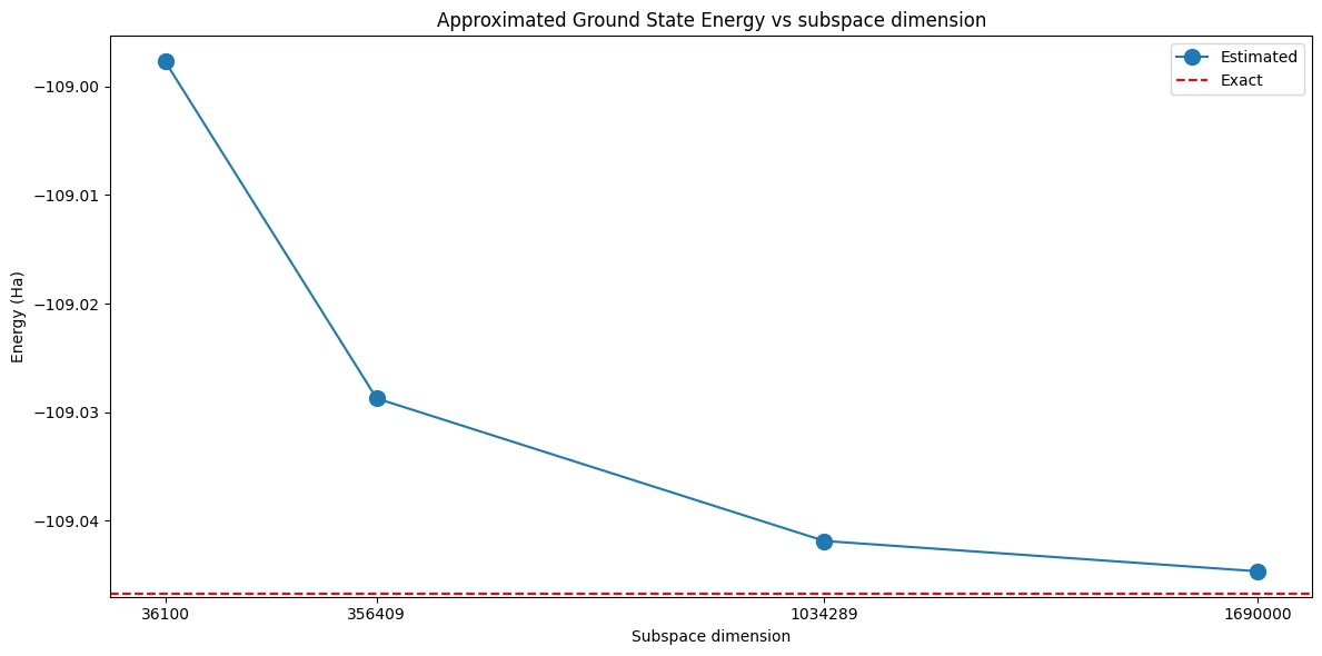
このプロットから、部分空間の次元を大きくするとより正確な結果が得られることがわかります。
import matplotlib.pyplot as plt

# Data for energies plot
x1 = subspace_dimensions
y1 = np.array(energies) + nuclear_repulsion_energy

fig, axs = plt.subplots(1, 1, figsize=(12, 6))

# Plot energies
axs.plot(x1, y1, marker=".", markersize=20, label="Estimated")
axs.set_xticks(x1)
axs.set_xticklabels(x1)
axs.axhline(y=exact_energy, color="red", linestyle="--", label="Exact")
axs.set_title("Approximated Ground State Energy vs subspace dimension")
axs.set_xlabel("Subspace dimension")
axs.set_ylabel("Energy (Ha)")
axs.legend()

plt.tight_layout()
plt.show()
max_dim で明示的な上限を設定する
上記のスイープでは、部分空間の次元は間接的にしか制御されていませんでした。samples_per_batch は各バッチに取り込まれるビット列の数を設定しますが、結果として得られる部分空間の次元は、それらのビット列に含まれる異なるスピンアルファ文字列とスピンベータ文字列の数で決まり、さらにサブサンプリングに使える配置のプールは、配置回復の反復ごとに増えていきます。そのため、上のグラフの横軸にある部分空間の次元は、私たちが選んだわけではない不規則な数値になっています。
diagonalize_fermionic_hamiltonian の max_dim 引数を使うと、次元を直接制限できます。これは各スピンセクターで保持する CI 文字列の数を制限します。部分空間は 2 つのセクターのデカルト積で張られるため、その次元は 2 つのセクターの次元の積になります。
-
max_dim=dは両方のセクターをd個の文字列に制限するため、部分空間の次元は最大でd ** 2です。 -
max_dim=(d_a, d_b)はスピンアルファとスピンベータのセクターを別々に制限するため、部分空間の次元は最大でd_a * d_bです。symmetrize_spin=Trueの場合、2 つの上限は等しくなければなりません。 -
デフォルトの
max_dim=Noneでは、制限は課されません。
バッチに上限を超える数の文字列が含まれる場合は、重要度の低いものから破棄されます。まず include_configurations で渡された文字列が保持され、次に前回の反復から引き継がれた文字列 (carryover_threshold を参照) が保持され、残りの枠はサンプリングされた回数の多い順にサンプリングされた文字列で埋められます。
max_dim は、固有状態ソルバーが実行する最大の対角化のサイズに上限を設けるため、ソルバーを実行時間とメモリの予算内に収める便利な方法です。samples_per_batch は余裕をもって大きく選び、部分空間をどこまで大きくしてよいかは max_dim に決めさせます。
以下では、samples_per_batch を固定し、max_dim を増やしながら、この調査を繰り返します。
list_max_dim = [100, 200, 400, 800]

# Use a generous number of samples per batch, so that max_dim is what limits
# the dimension of the subspace
samples_per_batch = 600

energies_max_dim = []
subspace_dimensions_max_dim = []

for max_dim in list_max_dim:
    result = diagonalize_fermionic_hamiltonian(
        hcore,
        eri,
        bit_array,
        samples_per_batch=samples_per_batch,
        norb=num_orbitals,
        nelec=(num_elec_a, num_elec_b),
        num_batches=num_batches,
        max_iterations=max_iterations,
        symmetrize_spin=True,
        max_dim=max_dim,
        seed=rng,
    )
    energies_max_dim.append(result.energy)
    subspace_dimensions_max_dim.append(
        int(np.prod(result.sci_state.amplitudes.shape))
    )

print(f"max_dim:            {list_max_dim}")
print(f"subspace dimension: {subspace_dimensions_max_dim}")
max_dim:            [100, 200, 400, 800]
subspace dimension: [10000, 40000, 160000, 640000]
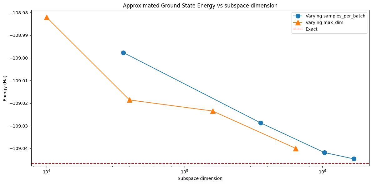
部分空間の次元は、どの実行でも正確に max_dim ** 2 になります。つまり、発見されたものではなく選択されたものです。両方のスイープを一緒にプロットすると、どちらの引数で到達したかにかかわらず、精度は部分空間の次元そのものによって決まることがわかります。ただし、2 本の曲線が完全に一致するとは限りません。max_dim を使った実行ではバッチごとに 600 個のビット列を取り出し、最も頻繁にサンプリングされた文字列を保持するため、最初からより少ないビット列をサンプリングしてその次元に到達した実行よりも、同じ次元でより良い配置の集合を保持できる場合があります。
fig, axs = plt.subplots(1, 1, figsize=(12, 6))

axs.plot(
    subspace_dimensions,
    np.array(energies) + nuclear_repulsion_energy,
    marker=".",
    markersize=20,
    label="Varying samples_per_batch",
)
axs.plot(
    subspace_dimensions_max_dim,
    np.array(energies_max_dim) + nuclear_repulsion_energy,
    marker="^",
    markersize=12,
    label="Varying max_dim",
)
axs.axhline(y=exact_energy, color="red", linestyle="--", label="Exact")
axs.set_xscale("log")
axs.ticklabel_format(axis="y", useOffset=False)
axs.set_title("Approximated Ground State Energy vs subspace dimension")
axs.set_xlabel("Subspace dimension")
axs.set_ylabel("Energy (Ha)")
axs.legend()

plt.tight_layout()
plt.show()