サンプルベースのクリロフ量子対角化によるフェルミオン格子模型のシミュレーション
使用量の目安: Heron r2 プロセッサで約9秒(注: これは推定値です。実際の実行時間は異なる場合があります。)
学習の成果
このチュートリアルを通じて、ユーザーは以下を理解できます:
- SQD Qiskitアドオンを使用して、量子処理ユニット(QPU)からサンプリングされたビット列を用いて格子モデルの基底状態エネルギーを近似する方法。
- ffsimを使用してフェルミオンシミュレーションの時間発展回路を構築する方法。
- 複数の回路からのサンプルを組み合わせてサンプルベースのクリロフ対角化(SQKD)アルゴリズムで後処理する方法。
前提知識
このチュートリアルを進める前に、以下のトピックに精通していることを推奨します:
背景
このチュートリアルでは、サンプルベースの量子対角化(SQD)を使用して、フェルミオン格子模型の基底状態エネルギーを推定する方法を示します。具体的には、金属中に埋め込まれた磁性不純物を記述するために使用される、一次元単一不純物アンダーソン模型(SIAM)を研究します。
このチュートリアルは、関連チュートリアル化学ハミルトニアンのサンプルベース量子対角化と類似したワークフローに従います。ただし、量子回路の構築方法に重要な違いがあります。もう一方のチュートリアルでは、数百万の相互作用項を持つ可能性のある化学ハミルトニアンに適したヒューリスティックな変分アンザッツを使用しています。一方、このチュートリアルでは、ハミルトニアンによる時間発展を近似する回路を使用します。このような回路は深くなる可能性があるため、このアプローチは格子模型への応用に適しています。これらの回路によって準備される状態ベクトルはクリロフ部分空間の基底を形成し、その結果、適切な仮定のもとでアルゴリズムは証明可能かつ効率的に基底状態に収束します。
このチュートリアルで使用されるアプローチは、SQDとクリロフ量子対角化(KQD)で使用される技術の組み合わせと見なすことができます。この組み合わせたアプローチは、サンプルベースのクリロフ量子対角化(SQKD)と呼ばれることがあります。KQD手法のチュートリアルについては、格子ハミルトニアンのクリロフ量子対角化を参照してください。
このチュートリアルは、論文"Quantum-Centric Algorithm for Sample-Based Krylov Diagonalization"に基づいており、詳細についてはそちらを参照してください。
単一不純物アンダーソン模型(SIAM)
一次元SIAMハミルトニアンは3つの項の和です:
ここで
ここで、 はスピン を持つ バスサイトのフェルミオン生成/消滅演算子、 は不純物モードの生成/消滅演算子、そして です。、、 はそれぞれホッピング、オンサイト、混成相互作用を記述する実数であり、 は化学ポテンシャルを指定する実数です。
このハミルトニアンは、一般的な相互作用電子ハミルトニアンの特殊なケースであることに注意してください。
ここで はフェルミオン生成・消滅演算子の二次形式である一体項から構成され、 は四次形式である二体項から構成されます。SIAMの場合、
であり、 はハミルトニアンの残りの項を含みます。ハミルトニアンをプログラム上で表現するために、行列 とテンソル を格納します。
位置基底と運動量基底
の近似的な並進対称性のため、基底状態が位置基底(上記でハミルトニアンが定義されている軌道基底)でスパースであることは期待できません。SQDの性能は、基底状態がスパースである場合、すなわち少数の計算基底状態にのみ有意な重みを持つ場合にのみ保証されます。基底状態のスパース性を向上させるために、 が対角化される軌道基底でシミュレーションを行います。この基底を運動量基底と呼びます。 は二次形式のフェルミオンハミルトニアンであるため、軌道回転によって効率的に対角化することができます。
ハミルトニアンによる近似的時間発展
ハミルトニアンによる時間発展を近似するために、二次のトロッター-鈴木分解を使用します。
ジョルダン-ウィグナー変換のもとで、 による時間発展は不純物サイトのスピンアップ軌道とスピンダウン軌道間の単一の CPhase ゲートに相当します。 は二次形式のフェルミオンハミルトニアンであるため、 による時間発展は軌道回転に相当します。
クリロフ基底状態 ( はクリロフ部分空間の次元)は、単一のトロッターステップの繰り返し適用によって形成されるため、
以下のSQDベースのワークフローでは、この回路セットからサンプリングを行い、得られたビット列の統合セットをSQDで後処理します。このアプローチは、関連チュートリアル化学ハミルトニアンのサンプルベース量子対角化で使用されているアプローチとは対照的であり、そちらでは単一のヒューリスティックな変分回路からサンプルが取得されます。
前提条件
このチュートリアルを開始する前に、以下がインストールされていることを確認してください:
- Qiskit SDK v1.0 以降、visualization サポート付き
- Qiskit Runtime v0.22 以降 (
pip install qiskit-ibm-runtime) - SQD Qiskit アドオン v0.11 以降 (
pip install qiskit-addon-sqd) - ffsim v0.0.72 以降 (
pip install ffsim)
小規模シミュレータの例
ステップ 1: 問題を量子回路にマッピングする
まず、位置基底でSIAMハミルトニアンを生成します。ハミルトニアンは行列 とテンソル で表現されます。次に、それを運動量基底に回転させます。位置基底では不純物を最初のサイトに配置しますが、運動量基底に回転する際には、他の軌道との相互作用を促進するために不純物を中央のサイトに移動させます。
# Added by doQumentation — required packages for this notebook
!pip install -q ffsim matplotlib numpy pyscf qiskit qiskit-addon-sqd qiskit-ibm-runtime scipy
import numpy as np
import pyscf.fci

def siam_hamiltonian(
    norb: int,
    hopping: float,
    onsite: float,
    hybridization: float,
    chemical_potential: float,
) -> tuple[np.ndarray, np.ndarray]:
    """Hamiltonian for the single-impurity Anderson model."""
    # Place the impurity on the first site
    impurity_orb = 0

    # One body matrix elements in the "position" basis
    h1e = np.zeros((norb, norb))
    np.fill_diagonal(h1e[:, 1:], -hopping)
    np.fill_diagonal(h1e[1:, :], -hopping)
    h1e[impurity_orb, impurity_orb + 1] = -hybridization
    h1e[impurity_orb + 1, impurity_orb] = -hybridization
    h1e[impurity_orb, impurity_orb] = chemical_potential

    # Two body matrix elements in the "position" basis
    h2e = np.zeros((norb, norb, norb, norb))
    h2e[impurity_orb, impurity_orb, impurity_orb, impurity_orb] = onsite

    return h1e, h2e

def momentum_basis(norb: int) -> np.ndarray:
    """Get the orbital rotation to change from the position to the momentum basis."""
    n_bath = norb - 1

    # Orbital rotation that diagonalizes the bath (non-interacting system)
    hopping_matrix = np.zeros((n_bath, n_bath))
    np.fill_diagonal(hopping_matrix[:, 1:], -1)
    np.fill_diagonal(hopping_matrix[1:, :], -1)
    _, vecs = np.linalg.eigh(hopping_matrix)

    # Expand to include impurity
    orbital_rotation = np.zeros((norb, norb))
    # Impurity is on the first site
    orbital_rotation[0, 0] = 1
    orbital_rotation[1:, 1:] = vecs

    # Move the impurity to the center
    new_index = n_bath // 2
    perm = np.r_[1 : (new_index + 1), 0, (new_index + 1) : norb]
    orbital_rotation = orbital_rotation[:, perm]

    return orbital_rotation

def rotated(
    h1e: np.ndarray, h2e: np.ndarray, orbital_rotation: np.ndarray
) -> tuple[np.ndarray, np.ndarray]:
    """Rotate the orbital basis of a Hamiltonian."""
    h1e_rotated = np.einsum(
        "ab,Aa,Bb->AB",
        h1e,
        orbital_rotation,
        orbital_rotation.conj(),
        optimize="greedy",
    )
    h2e_rotated = np.einsum(
        "abcd,Aa,Bb,Cc,Dd->ABCD",
        h2e,
        orbital_rotation,
        orbital_rotation.conj(),
        orbital_rotation,
        orbital_rotation.conj(),
        optimize="greedy",
    )
    return h1e_rotated, h2e_rotated

# Total number of spatial orbitals, including the bath sites and the impurity
# This should be an even number
norb = 8

# System is half-filled
nelec = (norb // 2, norb // 2)
# One orbital is the impurity, the rest are bath sites
n_bath = norb - 1

# Hamiltonian parameters
hybridization = 1.0
hopping = 1.0
onsite = 10.0
chemical_potential = -0.5 * onsite

# Generate Hamiltonian in position basis
h1e, h2e = siam_hamiltonian(
    norb=norb,
    hopping=hopping,
    onsite=onsite,
    hybridization=hybridization,
    chemical_potential=chemical_potential,
)

# Rotate to momentum basis
orbital_rotation = momentum_basis(norb)
h1e_momentum, h2e_momentum = rotated(h1e, h2e, orbital_rotation.T.conj())
# In the momentum basis, the impurity is placed in the center
impurity_index = n_bath // 2

# Use PySCF to compute the exact ground state energy
reference_energy, _ = pyscf.fci.direct_spin1.kernel(h1e, h2e, norb, nelec)
from typing import Sequence

import ffsim
import scipy
from qiskit import QuantumCircuit, QuantumRegister
from qiskit.circuit import CircuitInstruction, Qubit
from qiskit.circuit.library import CPhaseGate, XGate, XXPlusYYGate

def prepare_initial_state(qubits: Sequence[Qubit], norb: int, nocc: int):
    """Prepare initial state."""
    assert norb >= 8
    x_gate = XGate()
    rot = XXPlusYYGate(0.5 * np.pi, -0.5 * np.pi)
    for i in range(nocc):
        yield CircuitInstruction(x_gate, [qubits[i]])
        yield CircuitInstruction(x_gate, [qubits[norb + i]])
    for i in range(3):
        for j in range(nocc - i - 1, nocc + i, 2):
            yield CircuitInstruction(rot, [qubits[j], qubits[j + 1]])
            yield CircuitInstruction(
                rot, [qubits[norb + j], qubits[norb + j + 1]]
            )
    yield CircuitInstruction(rot, [qubits[j + 1], qubits[j + 2]])
    yield CircuitInstruction(
        rot, [qubits[norb + j + 1], qubits[norb + j + 2]]
    )

def trotter_step(
    qubits: Sequence[Qubit],
    time_step: float,
    one_body_evolution: np.ndarray,
    h2e: np.ndarray,
    impurity_index: int,
    norb: int,
):
    """A Trotter step."""
    # Assume the two-body interaction is just the on-site interaction of the impurity
    onsite = h2e[
        impurity_index, impurity_index, impurity_index, impurity_index
    ]
    # Two-body evolution for half the time
    yield CircuitInstruction(
        CPhaseGate(-0.5 * time_step * onsite),
        [qubits[impurity_index], qubits[norb + impurity_index]],
    )
    # One-body evolution for the full time
    yield CircuitInstruction(
        ffsim.qiskit.OrbitalRotationJW(norb, one_body_evolution), qubits
    )
    # Two-body evolution for half the time
    yield CircuitInstruction(
        CPhaseGate(-0.5 * time_step * onsite),
        [qubits[impurity_index], qubits[norb + impurity_index]],
    )

# Time step
time_step = 0.2
# Number of Krylov basis states
krylov_dim = 8

# Initialize circuit
qubits = QuantumRegister(2 * norb, name="q")
circuit = QuantumCircuit(qubits)

# Generate initial state
for instruction in prepare_initial_state(qubits, norb=norb, nocc=norb // 2):
    circuit.append(instruction)
circuit.measure_all()

# Create list of circuits, starting with the initial state circuit
circuits = [circuit.copy()]

# Add time evolution circuits to the list
one_body_evolution = scipy.linalg.expm(-1j * time_step * h1e_momentum)
for i in range(krylov_dim - 1):
    # Remove measurements
    circuit.remove_final_measurements()
    # Append another Trotter step
    for instruction in trotter_step(
        qubits,
        time_step,
        one_body_evolution,
        h2e_momentum,
        impurity_index,
        norb,
    ):
        circuit.append(instruction)
    # Measure qubits
    circuit.measure_all()
    # Add a copy of the circuit to the list
    circuits.append(circuit.copy())
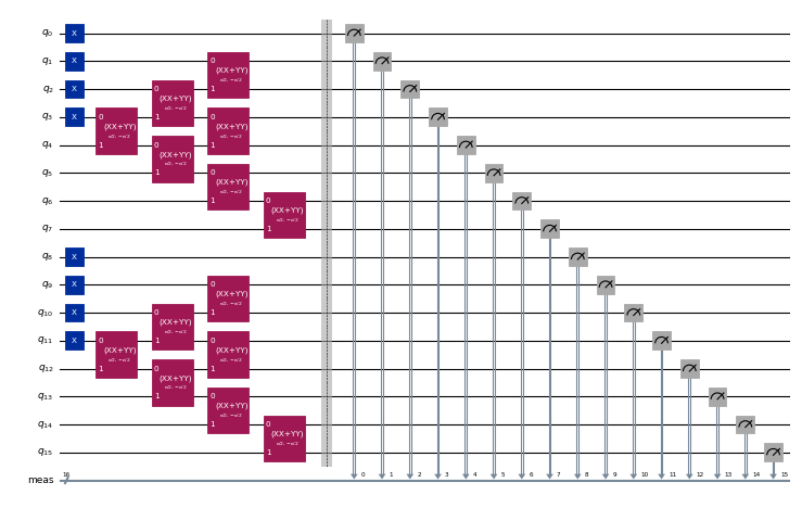
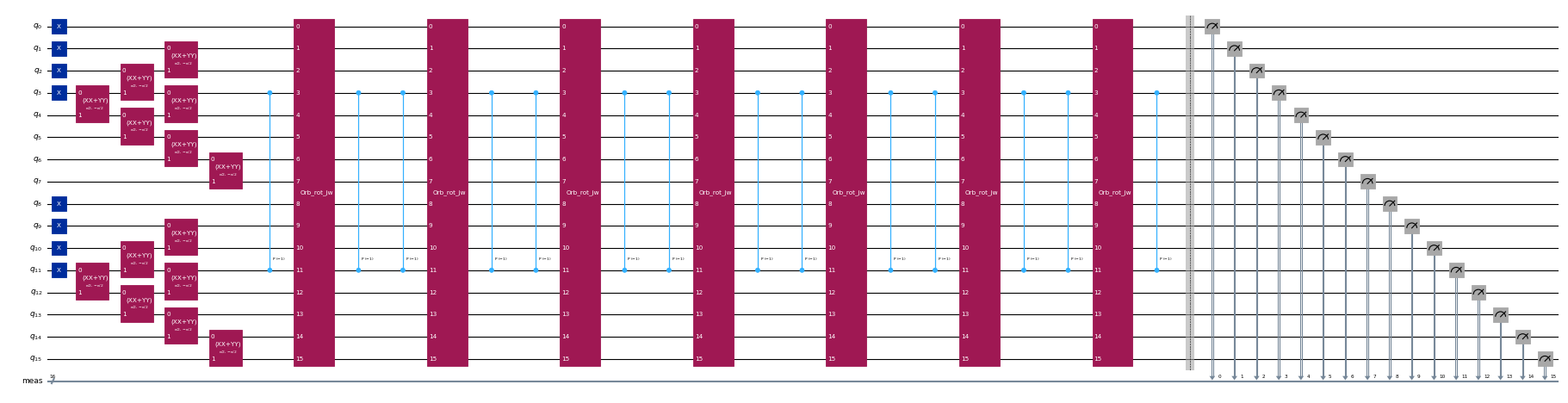
次に、クリロフ基底状態を生成するための回路を作成します。 各スピン種について、初期状態 は、状態 からフェルミ準位に最も近い3つの電子を最も近い4つの空きモードに励起するすべての可能な励起の重ね合わせとして与えられ、7つの XXPlusYYGate の適用によって実現されます。 時間発展した状態は、二次のトロッターステップの逐次適用によって生成されます。
この模型と回路の設計方法のより詳細な説明については、"Quantum-Centric Algorithm for Sample-Based Krylov Diagonalization"を参照してください。
circuits[0].draw("mpl", scale=0.4, fold=-1)
circuits[-1].draw("mpl", scale=0.4, fold=-1)
ステップ 2: 量子実行に向けた問題の最適化
次に、ターゲットハードウェアに合わせて回路を最適化します。ここでは、指定された量子ビット数と時間発展回路が自然に分解できるゲートセットを持つ汎用バックエンドを作成します。
from qiskit.providers.fake_provider import GenericBackendV2

backend = GenericBackendV2(
    2 * norb, basis_gates=["cp", "xx_plus_yy", "p", "x"]
)
次に、Qiskitを使用して回路をターゲットバックエンドにトランスパイルします。
from qiskit.transpiler import generate_preset_pass_manager

pass_manager = generate_preset_pass_manager(
    optimization_level=3, backend=backend
)
isa_circuits = pass_manager.run(circuits)
ステップ 3: Qiskitプリミティブを使用した実行
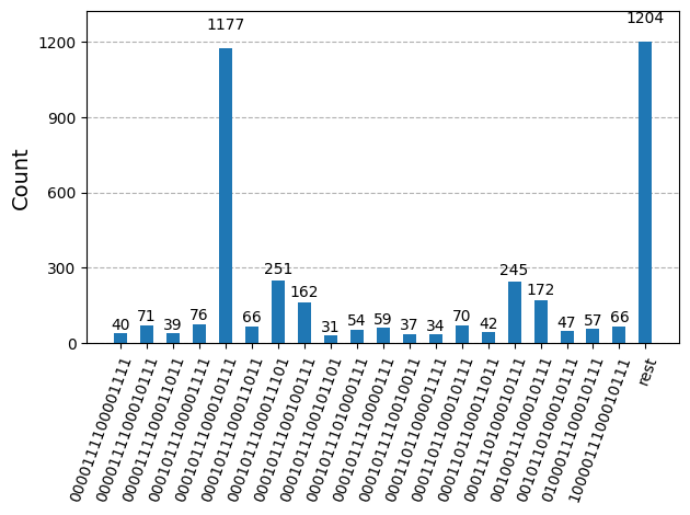
ハードウェア実行に向けて回路を最適化した後、ターゲットハードウェア上で回路を実行し、基底状態エネルギー推定のためのサンプルを収集する準備が整いました。Samplerプリミティブを使用して各回路からビット列をサンプリングした後、すべての結果を単一のカウント辞書にまとめ、最も頻繁にサンプリングされた上位20個のビット列をプロットします。
from qiskit.visualization import plot_histogram
from qiskit.primitives import StatevectorSampler

# Sample from the circuits
sampler = StatevectorSampler()
job = sampler.run(isa_circuits, shots=500)
from qiskit.primitives import BitArray

# Combine the shots from the individual Trotter circuits
bit_array = BitArray.concatenate_shots(
    [result.data.meas for result in job.result()]
)

plot_histogram(bit_array.get_counts(), number_to_keep=20)
ステップ 4: 後処理と結果の所望の古典フォーマットへの変換
ここでは、diagonalize_fermionic_hamiltonian関数を使用してSQDアルゴリズムを実行します。この関数の引数の説明については、APIドキュメントを参照してください。
from qiskit_addon_sqd.fermion import (
    SCIResult,
    diagonalize_fermionic_hamiltonian,
)

# List to capture intermediate results
result_history = []

def callback(results: list[SCIResult]):
    result_history.append(results)
    iteration = len(result_history)
    print(f"Iteration {iteration}")
    for i, result in enumerate(results):
        print(f"\tSubsample {i}")
        print(f"\t\tEnergy: {result.energy}")
        print(
            f"\t\tSubspace dimension: {np.prod(result.sci_state.amplitudes.shape)}"
        )

rng = np.random.default_rng(24)
result = diagonalize_fermionic_hamiltonian(
    h1e_momentum,
    h2e_momentum,
    bit_array,
    samples_per_batch=100,
    norb=norb,
    nelec=nelec,
    num_batches=3,
    max_iterations=5,
    symmetrize_spin=True,
    callback=callback,
    seed=rng,
)
Iteration 1
	Subsample 0
		Energy: -13.4222953188441
		Subspace dimension: 529
	Subsample 1
		Energy: -13.42237556285828
		Subspace dimension: 784
	Subsample 2
		Energy: -13.422045397387413
		Subspace dimension: 529
Iteration 2
	Subsample 0
		Energy: -13.422379583305478
		Subspace dimension: 900
	Subsample 1
		Energy: -13.422376197704326
		Subspace dimension: 841
	Subsample 2
		Energy: -13.422421162849295
		Subspace dimension: 1089
Iteration 3
	Subsample 0
		Energy: -13.422421164670345
		Subspace dimension: 1156
	Subsample 1
		Energy: -13.422421492737689
		Subspace dimension: 1156
	Subsample 2
		Energy: -13.422421205869572
		Subspace dimension: 1156
Iteration 4
	Subsample 0
		Energy: -13.422421494558726
		Subspace dimension: 1225
	Subsample 1
		Energy: -13.422421492737689
		Subspace dimension: 1156
	Subsample 2
		Energy: -13.422421492737689
		Subspace dimension: 1156
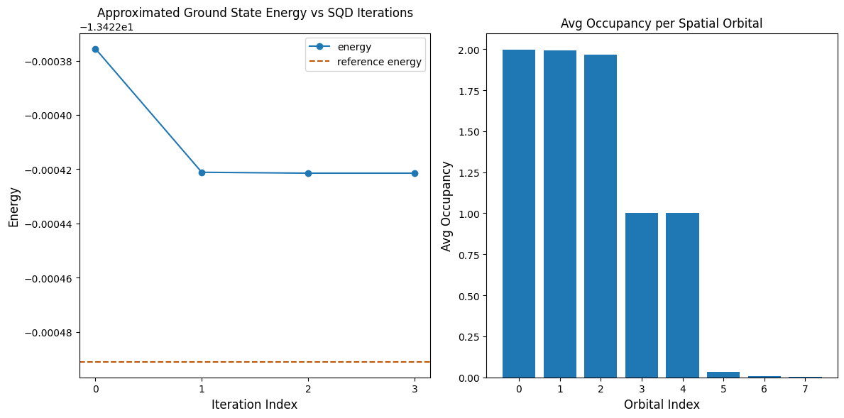
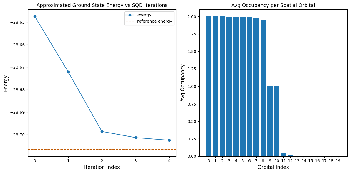
以下のコードセルは結果をプロットします。最初のプロットは配置回復イテレーション数の関数として計算されたエネルギーを示し、2番目のプロットは最終イテレーション後の各空間軌道の平均占有数を示します。この問題は非常に小規模なので、最初のイテレーションでも正確なエネルギーに非常に近い値が得られます(y軸のスケールに注目してください)。
import matplotlib.pyplot as plt

min_es = [
    min(result, key=lambda res: res.energy).energy
    for result in result_history
]
min_id, min_e = min(enumerate(min_es), key=lambda x: x[1])

# Data for energies plot
x1 = range(len(result_history))

# Data for avg spatial orbital occupancy
y2 = np.sum(result.orbital_occupancies, axis=0)
x2 = range(len(y2))

fig, axs = plt.subplots(1, 2, figsize=(12, 6))

# Plot energies
axs[0].plot(x1, min_es, label="energy", marker="o")
axs[0].set_xticks(x1)
axs[0].set_xticklabels(x1)
axs[0].axhline(
    y=reference_energy,
    color="#BF5700",
    linestyle="--",
    label="reference energy",
)
axs[0].set_title("Approximated Ground State Energy vs SQD Iterations")
axs[0].set_xlabel("Iteration Index", fontdict={"fontsize": 12})
axs[0].set_ylabel("Energy", fontdict={"fontsize": 12})
axs[0].legend()

# Plot orbital occupancy
axs[1].bar(x2, y2, width=0.8)
axs[1].set_xticks(x2)
axs[1].set_xticklabels(x2)
axs[1].set_title("Avg Occupancy per Spatial Orbital")
axs[1].set_xlabel("Orbital Index", fontdict={"fontsize": 12})
axs[1].set_ylabel("Avg Occupancy", fontdict={"fontsize": 12})

print(f"Reference energy: {reference_energy:.5f}")
print(f"SQD energy: {min_e:.5f}")
print(f"Absolute error: {abs(min_e - reference_energy):.5f}")
plt.tight_layout()
plt.show()
Reference energy: -13.42249
SQD energy: -13.42242
Absolute error: 0.00007
エネルギーの確認
SQDによって返されるエネルギーは、真の基底状態エネルギーの上界であることが保証されています。SQDは基底状態を近似する状態ベクトルの係数も返すため、エネルギーの値を検証することができます。以下のコードセルに示すように、1粒子および2粒子の縮約密度行列を使用して状態ベクトルからエネルギーを計算できます。
rdm1 = result.sci_state.rdm(rank=1, spin_summed=True)
rdm2 = result.sci_state.rdm(rank=2, spin_summed=True)

energy = np.sum(h1e_momentum * rdm1) + 0.5 * np.sum(h2e_momentum * rdm2)

print(f"Recomputed energy: {energy:.5f}")
Recomputed energy: -13.42242
大規模ハードウェアの例
次に、実際のQPU上でより大きな例を実行します。 参照エネルギーとしては、別途実行されたDMRG計算の結果を使用します。
from qiskit_ibm_runtime import SamplerV2 as Sampler
from qiskit_ibm_runtime import QiskitRuntimeService

# Model parameters
norb = 20
nelec = (norb // 2, norb // 2)
n_bath = norb - 1
hybridization = 1.0
hopping = 1.0
onsite = 10.0
chemical_potential = -0.5 * onsite

# Generate Hamiltonian and orbital rotation
h1e, h2e = siam_hamiltonian(
    norb=norb,
    hopping=hopping,
    onsite=onsite,
    hybridization=hybridization,
    chemical_potential=chemical_potential,
)
orbital_rotation = momentum_basis(norb)
h1e_momentum, h2e_momentum = rotated(h1e, h2e, orbital_rotation.T.conj())
impurity_index = n_bath // 2

# Set reference energy to DMRG value computed separately
reference_energy = -28.70659686

# Algorithm parameters
time_step = 0.2
krylov_dim = 8

# Construct circuits
qubits = QuantumRegister(2 * norb, name="q")
circuit = QuantumCircuit(qubits)
for instruction in prepare_initial_state(qubits, norb=norb, nocc=norb // 2):
    circuit.append(instruction)
circuit.measure_all()
circuits = [circuit.copy()]
one_body_evolution = scipy.linalg.expm(-1j * time_step * h1e_momentum)
for i in range(krylov_dim - 1):
    circuit.remove_final_measurements()
    for instruction in trotter_step(
        qubits,
        time_step,
        one_body_evolution,
        h2e_momentum,
        impurity_index,
        norb,
    ):
        circuit.append(instruction)
    circuit.measure_all()
    circuits.append(circuit.copy())

# Initialize hardware backend
service = QiskitRuntimeService()
backend = service.least_busy(
    operational=True, simulator=False, min_num_qubits=127
)
print(f"Using backend {backend.name}")

# Transpile to backend
pass_manager = generate_preset_pass_manager(
    optimization_level=3, backend=backend
)
isa_circuits = pass_manager.run(circuits)

# Sample from the circuits
sampler = Sampler(backend)
sampler.options.environment.job_tags = ["TUT_SKQD"]
job = sampler.run(isa_circuits, shots=500)

# Combine the shots from the individual Trotter circuits
bit_array = BitArray.concatenate_shots(
    [result.data.meas for result in job.result()]
)

# Run configuration recovery and diagonalization
result_history = []

def callback(results: list[SCIResult]):
    result_history.append(results)
    iteration = len(result_history)
    print(f"Iteration {iteration}")
    for i, result in enumerate(results):
        print(f"\tSubsample {i}")
        print(f"\t\tEnergy: {result.energy}")
        print(
            f"\t\tSubspace dimension: {np.prod(result.sci_state.amplitudes.shape)}"
        )

rng = np.random.default_rng(24)
result = diagonalize_fermionic_hamiltonian(
    h1e_momentum,
    h2e_momentum,
    bit_array,
    samples_per_batch=100,
    norb=norb,
    nelec=nelec,
    num_batches=3,
    max_iterations=5,
    symmetrize_spin=True,
    callback=callback,
    seed=rng,
)

# Plot results
min_es = [
    min(result, key=lambda res: res.energy).energy
    for result in result_history
]
min_id, min_e = min(enumerate(min_es), key=lambda x: x[1])
x1 = range(len(result_history))
y2 = np.sum(result.orbital_occupancies, axis=0)
x2 = range(len(y2))
fig, axs = plt.subplots(1, 2, figsize=(12, 6))
axs[0].plot(x1, min_es, label="energy", marker="o")
axs[0].set_xticks(x1)
axs[0].set_xticklabels(x1)
axs[0].axhline(
    y=reference_energy,
    color="#BF5700",
    linestyle="--",
    label="reference energy",
)
axs[0].set_title("Approximated Ground State Energy vs SQD Iterations")
axs[0].set_xlabel("Iteration Index", fontdict={"fontsize": 12})
axs[0].set_ylabel("Energy", fontdict={"fontsize": 12})
axs[0].legend()
axs[1].bar(x2, y2, width=0.8)
axs[1].set_xticks(x2)
axs[1].set_xticklabels(x2)
axs[1].set_title("Avg Occupancy per Spatial Orbital")
axs[1].set_xlabel("Orbital Index", fontdict={"fontsize": 12})
axs[1].set_ylabel("Avg Occupancy", fontdict={"fontsize": 12})
print(f"Reference energy: {reference_energy:.5f}")
print(f"SQD energy: {min_e:.5f}")
print(f"Absolute error: {abs(min_e - reference_energy):.5f}")
plt.tight_layout()
plt.show()
Using backend ibm_boston
Iteration 1
	Subsample 0
		Energy: -28.63965951544449
		Subspace dimension: 9801
	Subsample 1
		Energy: -28.625588929202006
		Subspace dimension: 9409
	Subsample 2
		Energy: -28.647371834135498
		Subspace dimension: 8281
Iteration 2
	Subsample 0
		Energy: -28.67213260849567
		Subspace dimension: 29584
	Subsample 1
		Energy: -28.670340686158816
		Subspace dimension: 27225
	Subsample 2
		Energy: -28.669976379525988
		Subspace dimension: 31329
Iteration 3
	Subsample 0
		Energy: -28.68622875601382
		Subspace dimension: 36100
	Subsample 1
		Energy: -28.698569623143126
		Subspace dimension: 34225
	Subsample 2
		Energy: -28.694848533971882
		Subspace dimension: 33856
Iteration 4
	Subsample 0
		Energy: -28.69883392844593
		Subspace dimension: 42025
	Subsample 1
		Energy: -28.701289495200996
		Subspace dimension: 38025
	Subsample 2
		Energy: -28.699319594978245
		Subspace dimension: 45369
Iteration 5
	Subsample 0
		Energy: -28.701936886834154
		Subspace dimension: 51076
	Subsample 1
		Energy: -28.702468711812013
		Subspace dimension: 53824
	Subsample 2
		Energy: -28.702298147575938
		Subspace dimension: 52900
Reference energy: -28.70660
SQD energy: -28.70247
Absolute error: 0.00413
次のステップ
この研究に興味を持たれた方は、以下の資料もご覧ください:
- 化学ハミルトニアンのサンプルベース量子対角化 - トロッター回路の代わりにヒューリスティックな変分アンザッツを使用した関連チュートリアル
- 格子ハミルトニアンのクリロフ量子対角化 - KQD手法に関するチュートリアル
- SQDアドオンAPIドキュメント -
diagonalize_fermionic_hamiltonian関数のリファレンス - Quantum-Centric Algorithm for Sample-Based Krylov Diagonalization - このチュートリアルの基となった論文