最適化マッパーQiskitアドオンによるQAOAのウォームスタート

使用時間の目安: Heron r3で9分(注: これはあくまで目安です。実際の実行時間は異なる場合があります。)

学習成果

• qiskit-addon-opt-mapperを使用してmax-cut問題を量子二次非制約二値最適化(QUBO)定式化にマッピングする方法

• シミュレーター上で標準QAOAを実装し実行する方法

• 二次計画(QP)緩和を計算し、ウォームスタートCircuitを構築することによりWS-QAOAを適用する方法

• 標準QAOAとWS-QAOAのエネルギー収束と解の品質を比較する方法

前提条件

• QAOAチュートリアル

• 高度なQAOAチュートリアル

背景

量子近似最適化アルゴリズム(QAOA)は、max-cutや一般的なQUBO定式化などの組み合わせ最適化問題を解くために設計されたハイブリッド量子古典アルゴリズムです。Qiskitにおける QAOA の基礎的な導入については、QAOAチュートリアルを、より高度なCircuit構築手法については、高度なQAOAチュートリアルを参照してください。

標準QAOAでは:

• 初期状態は一様重ね合わせ$|+\rangle^{\otimes n}$です。
• 変分パラメーターはランダムに初期化されます。
• 古典最適化アルゴリズムがコスト関数を最小化するパラメーターを探索します。

しかし、実用的な問題サイズとノイズのある量子ハードウェアでは、ランダム初期化は収束の遅さ、局所最小値の悪化、そして最適化コストの増加につながる可能性があります。

ウォームスタートQAOA(WS-QAOA)は、古典的な最適化の知見を量子Circuitに直接組み込むことでこれを改善します。このチュートリアルは、Egger、Mareček、WoernerによってWarm-starting quantum optimizationで紹介された手法に従っています。主なアイデアは以下の通りです。

1. 元の二値問題の連続緩和を解く($\{0,1\}^n$の代わりに$[0,1]^n$上の二次計画)。

2. $Y$回転角$\theta_i = 2\arcsin(\sqrt{c^*_i})$を使用して、緩和された解$c^*_i \in [0,1]$をカスタム初期状態にエンコードし、Qubit $i$が$|1\rangle$を測定する確率が$c^*_i$である状態から開始するようにします。

3. 標準の$X$-mixerを置き換えて、その基底状態がウォームスタート初期状態であるカスタムmixerを使用し、アルゴリズムが古典解の近くから開始し、近傍を探索できるようにします。

正則化パラメーター$\varepsilon \in [0, 0.5]$は、到達可能性の問題を避けるために$c^*_i$を0と1から遠ざけてクリップします。$|0\rangle$または$|1\rangle$に初期化されたQubitは、コストHamiltonianによって動かすことができません。$\varepsilon = 0.5$では、WS-QAOAは正確に標準QAOAに帰着します。

問題のモデル化にはqiskit-addon-opt-mapperパッケージを使用します。そのMaxcutアプリケーションクラスは、グラフから直接QUBOを構築し、そのコンバーターとトランスレーターは結果として得られる問題を量子Hamiltonianにマッピングします。

要件

このチュートリアルを始める前に、以下がインストールされていることを確認してください。

• Qiskit SDK v2.0以降(可視化サポート付き)

• Qiskit Runtime v0.43以降(pip install qiskit-ibm-runtime)

• 最適化マッパーQiskitアドオン(pip install qiskit-addon-opt-mapper)

• SciPy (pip install scipy)

• NetworkX (pip install networkx)

セットアップ

このチュートリアル全体を通して使用する必要なライブラリをすべてインポートし、ヘルパー関数を定義します。

# Added by doQumentation — required packages for this notebook
!pip install -q matplotlib networkx numpy qiskit qiskit-addon-opt-mapper qiskit-ibm-runtime scipy

import numpy as np
import matplotlib.pyplot as plt
import networkx as nx
from scipy.optimize import minimize

from qiskit.circuit import QuantumCircuit, ParameterVector
from qiskit.circuit.library import qaoa_ansatz
from qiskit.quantum_info import Statevector
from qiskit.primitives import StatevectorEstimator, StatevectorSampler
from qiskit.transpiler.preset_passmanagers import generate_preset_pass_manager
from qiskit_ibm_runtime import (
    QiskitRuntimeService,
    Session,
    EstimatorOptions,
    EstimatorV2 as Estimator,
    SamplerV2 as Sampler,
)

from qiskit_addon_opt_mapper.applications import Maxcut
from qiskit_addon_opt_mapper.converters import OptimizationProblemToQubo
from qiskit_addon_opt_mapper.translators import to_ising

小規模シミュレーター例

実行例として、重み付きグラフ上の小さなmax-cut問題を使用します。max-cutは次のように問います。エッジの重み$w_{ij}$を持つグラフ$G=(V,E)$が与えられたとき、カットを横切るエッジの総重みを最大化する、頂点を2つの集合$S$と$\bar{S}$に分割するパーティションを見つけよ。

QUBO最小化問題として、max-cutは次のように書けます。 $\min_{x \in \{0,1\}^n} -\sum_{(i,j) \in E} w_{ij}(x_i + x_j - 2x_i x_j)$

シミュレーター上で扱いやすいように、4ノードのグラフを使用します。

ステップ1: 古典入力を量子問題にマッピングする

qiskit-addon-opt-mapperのMaxcutアプリケーションクラスを使用してmax-cut問題を定義します。これはグラフから直接QUBO定式化を構築します。次に、それをQUBOに変換し、QAOAに適したIsing Hamiltonian(SparsePauliOp)に変換します。また、二値制約$x_i \in \{0,1\}$を$x_i \in [0,1]$に置き換えて、QUBOの連続緩和を解き、ウォームスタート初期点$c^*$を得ます。

# Define a 4-node weighted graph for the max-cut problem
n_nodes = 4
edges = [(0, 1, 1.0), (0, 2, 1.0), (1, 2, 1.0), (1, 3, 1.0), (2, 3, 1.0)]

G = nx.Graph()
G.add_nodes_from(range(n_nodes))
G.add_weighted_edges_from(edges)

pos = nx.spring_layout(G, seed=42)
edge_labels = {(u, v): d["weight"] for u, v, d in G.edges(data=True)}

fig, ax = plt.subplots(figsize=(4, 3))
nx.draw(G, pos, with_labels=True, node_color="lightblue", ax=ax)
nx.draw_networkx_edge_labels(G, pos, edge_labels=edge_labels, ax=ax)
ax.set_title("Max-Cut graph")
plt.tight_layout()
plt.show()

このグラフには5つのエッジがあります。最適なmax-cutは、ノードを$S = \{0, 3\}$と$\bar{S} = \{1, 2\}$(またはその補集合)に分割し、5つのエッジのうち4つを切断してカット値4を得ます。

# Build the max-cut problem directly from the NetworkX graph using the
# Maxcut application class. Internally it constructs the QUBO
#   minimize  -sum_{(i,j) in E} w_ij * (x_i + x_j - 2*x_i*x_j)
# (each edge contributes -w to the linear terms and +2w to the quadratic
# term), so we get the same OptimizationProblem without the boilerplate.
maxcut = Maxcut(G)
prob = maxcut.to_optimization_problem()
print(prob.prettyprint())

Problem name: Max-cut

Maximize
  -2*x_0*x_1 - 2*x_0*x_2 - 2*x_1*x_2 - 2*x_1*x_3 - 2*x_2*x_3 + 2*x_0 + 3*x_1
  + 3*x_2 + 2*x_3

Subject to
  No constraints

  Binary variables (4)
    x_0 x_1 x_2 x_3

MaxcutクラスはQUBOの構築をラップしているため、手動でmax-cutの目的関数を展開する必要はありません。表示される目的関数は、各変数の線形係数(各変数がカットに個別に寄与する量)と各交差項の二次係数(2つの隣接ノードを同じ側に置くことに対するペナルティ)を示します。to_optimization_problem()によって返される基礎となるOptimizationProblemは、二値、整数、連続、スピン変数をサポートし、次のステップで使用されるコンバーターとトランスレーターが期待するのと同じオブジェクトです。

# Convert the OptimizationProblem to a QUBO, then translate to an Ising Hamiltonian
#
# The substitution x_i = (1 - z_i)/2  maps binary variables to spin operators,
# yielding a Hamiltonian H_C = sum_i h_i Z_i + sum_{i<j} J_ij Z_i Z_j + constant.
# QAOA minimizes <H_C> to find the ground state, which encodes the optimal cut.
converter = OptimizationProblemToQubo()
qubo = converter.convert(prob)

cost_operator, offset = to_ising(qubo)
n_qubits = cost_operator.num_qubits

print(f"Cost Hamiltonian H_C ({n_qubits} qubits):")
print(cost_operator)
print(f"\nOffset (constant shift): {offset}")
print("  QUBO value = Ising energy + offset")

Cost Hamiltonian H_C (4 qubits):
SparsePauliOp(['IIZZ', 'IZIZ', 'IZZI', 'ZIZI', 'ZZII'],
              coeffs=[0.5+0.j, 0.5+0.j, 0.5+0.j, 0.5+0.j, 0.5+0.j])

Offset (constant shift): -2.5
  QUBO value = Ising energy + offset

to_isingトランスレーターは、$H_C$を表すSparsePauliOpと、$\text{QUBO value} = \langle H_C \rangle + \text{offset}$を満たすスカラーoffsetを返します。すべての重みが単位である今回のmax-cut問題では、すべてのQubitについて$h_i = 0$です($x_i \to z_i$の代入後、線形項に関してグラフは対称です)。また、各エッジは強度$+0.5$の$Z_i Z_j$結合を寄与します。$H_C$の最小固有値は最大カットに対応します。

# Solve the continuous (QP) relaxation to obtain the warm-start point c*
#
# The QP relaxation replaces the binary constraint x_i in {0,1} with x_i in [0,1]
# and minimizes the same quadratic objective. Its solution c*_i gives the
# probability that variable i should be 1 according to the classical relaxation.
#
# The max-cut QUBO has a non-convex quadratic matrix (negative eigenvalues),
# so the relaxed problem has multiple local minima. A naive single start from
# [0.5,...,0.5] converges to the symmetric saddle point c* = [0.5,...,0.5],
# which carries no useful structural information about the problem.
# Multi-start optimization is used to reliably find the global minimum.
Q = qubo.objective.quadratic.to_array(symmetric=True)
mu = qubo.objective.linear.to_array()

def qp_objective(x_cont):
    """Continuous relaxation of the QUBO objective."""
    return x_cont @ Q @ x_cont + mu @ x_cont + qubo.objective.constant

bounds = [(0.0, 1.0)] * n_qubits

rng = np.random.default_rng(42)
best_val = np.inf
c_star = None
for _ in range(200):
    x0 = rng.uniform(0.0, 1.0, n_qubits)
    result = minimize(qp_objective, x0, method="L-BFGS-B", bounds=bounds)
    if result.fun < best_val:
        best_val = result.fun
        c_star = result.x

print(f"QP relaxation solution c* = {np.round(c_star, 4)}")
print(f"QP objective value        = {best_val:.4f}")

QP relaxation solution c* = [1. 0. 0. 1.]
QP objective value        = -4.0000

マルチスタートソルバーは、実際の最適な二値解である$c^* = [1, 0, 0, 1]$(またはその補集合$[0, 1, 1, 0]$)を見つけます。この問題ではQP緩和がタイトであり、連続最小値が整数最適値と一致します。つまり、緩和は最良のカットを即座に特定します。ステップ2で$\varepsilon = 0.25$による正則化を行った後、この解はウォームスタート初期状態にエンコードされます。

ステップ2: 量子ハードウェア実行向けに問題を最適化する

2つのQAOA Circuitを構築し、QP解からウォームスタート角度を準備します。

標準QAOAは、一様重ね合わせ$|+\rangle^{\otimes n}$を初期状態として使用し、標準の$X$-mixer $H_M = -\sum_i X_i$を使用します。これは各レイヤーで$\prod_i R_X(-2\beta)$として実装されます。

[1]による**ウォームスタートQAOA(WS-QAOA)**は、Qubit $i$ごとに2つの構造的な変更を行います。

• 初期状態: $R_Y(\theta_i)|0\rangle$、$\theta_i = 2\arcsin(\sqrt{c^*_i})$。これにより、$|1\rangle$を測定する確率が$c^*_i$に等しくなります。
• カスタムmixer: $R_Y(\theta_i)\, R_Z(-2\beta)\, R_Y(-\theta_i)$。これは$R_Y(\theta_i)|0\rangle$を基底状態として持ちます。これは、WS-QAOAが自身のmixerの基底状態から始まることを意味し、標準QAOAが$|+\rangle$と$X$-mixerで満たすのと同じ性質です。

レイヤーに関する注記: p=1(単一のQAOAレイヤー)では、標準QAOAは解析的に、三角形を含むグラフ上で最適エネルギーの約49%に制限されます(このグラフには三角形0-1-2があります)。ウォームスタートは、解の事前知識を初期状態に直接エンコードすることで、この制限を回避します。

# Number of QAOA layers (each layer = one cost unitary + one mixer unitary)
p = 1

# Regularization: clip c* to [epsilon, 1-epsilon] so no qubit is initialized
# in |0> or |1>, which would freeze it under the cost Hamiltonian.
epsilon = 0.25

c_clipped = np.clip(c_star, epsilon, 1 - epsilon)
thetas = 2 * np.arcsin(np.sqrt(c_clipped))

print(f"Continuous relaxation c*  = {np.round(c_star, 4)}")
print(f"After regularization      = {np.round(c_clipped, 4)}")
print(f"Warm-start angles theta   = {np.round(thetas, 4)} radians")
print()
print("Angle interpretation:")
print("  theta = 0      <->  c* = 0   (qubit points toward |0>)")
print(
    "  theta = pi/2   <->  c* = 0.5 (qubit in equal superposition, like |+>)"
)
print("  theta = pi     <->  c* = 1   (qubit points toward |1>)")

Continuous relaxation c*  = [1. 0. 0. 1.]
After regularization      = [0.75 0.25 0.25 0.75]
Warm-start angles theta   = [2.0944 1.0472 1.0472 2.0944] radians

Angle interpretation:
  theta = 0      <->  c* = 0   (qubit points toward |0>)
  theta = pi/2   <->  c* = 0.5 (qubit in equal superposition, like |+>)
  theta = pi     <->  c* = 1   (qubit points toward |1>)

クリッピング後、$c^* = 1$は$1 - \varepsilon = 0.75$に、$c^* = 0$は$\varepsilon = 0.25$になります。結果として得られる角度$\theta \approx [2.09, 1.05, 1.05, 2.09]$ラジアンは、Qubit0と3を$|1\rangle$に強く回転させ、Qubit1と2を$|0\rangle$に回転させることで、最適なカットの構造を初期量子状態に直接エンコードします。

def apply_cost_unitary(qc, cost_op, gamma):
    """Apply exp(-i * gamma * H_C) to the circuit.

    Each Pauli term in H_C contributes a rotation gate:
      - Single-Z term h_i * Z_i  ->  RZ(2 * gamma * h_i) on qubit i
      - Two-Z term J_ij * Z_i Z_j  ->  CNOT, RZ(2 * gamma * J_ij), CNOT
    """
    for pauli_term, coeff in zip(cost_op.paulis, cost_op.coeffs):
        indices = [
            j for j, q in enumerate(pauli_term.to_label()[::-1]) if q == "Z"
        ]
        if len(indices) == 1:
            qc.rz(2 * gamma * coeff.real, indices[0])
        elif len(indices) == 2:
            qc.cx(indices[0], indices[1])
            qc.rz(2 * gamma * coeff.real, indices[1])
            qc.cx(indices[0], indices[1])

def build_ws_qaoa(cost_op, n_layers, n_qubits, thetas):
    """WS-QAOA: warm-start initial state + custom per-qubit mixer.

    Per Egger et al. (2021) Eq. (1)-(2):
      Initial state per qubit i:  R_Y(theta_i) |0>
      Mixer gate per qubit i:     R_Y(theta_i) R_Z(-2*beta) R_Y(-theta_i)
    """
    gammas = ParameterVector("γ", n_layers)
    betas = ParameterVector("β", n_layers)
    qc = QuantumCircuit(n_qubits)
    for i, theta in enumerate(thetas):
        qc.ry(theta, i)  # warm-start initial state
    for k in range(n_layers):
        apply_cost_unitary(qc, cost_op, gammas[k])
        for i, theta in enumerate(thetas):
            qc.ry(theta, i)
            qc.rz(-2 * betas[k], i)
            qc.ry(-theta, i)
    return qc, gammas, betas

# Standard QAOA via the Qiskit built-in helper:
# qaoa_ansatz prepares |+>^n, then alternates exp(-i*gamma*H_C) with the
# default X-mixer for `reps` layers. The returned circuit exposes the
# variational parameters via std_qc.parameters.
std_qc = qaoa_ansatz(cost_operator, reps=p)

# WS-QAOA: keep the custom builder. The per-qubit mixer
# R_Y(theta_i) R_Z(-2*beta) R_Y(-theta_i) is implemented as an explicit gate
# sequence rather than as a SparsePauliOp, so we construct the circuit
# directly to stay close to the Egger et al. (2021) formulation.
ws_qc, ws_gammas, ws_betas = build_ws_qaoa(cost_operator, p, n_qubits, thetas)

標準アンサッツについては、qaoa_ansatzに委ねます。これは$|+\rangle^{\otimes n}$を構築し、コストユニタリを適用し、各repsレイヤーにデフォルトの$X$-mixerを適用します。WS-QAOAについては、Qubitごとのmixer $R_Y(\theta)\,R_Z(-2\beta)\,R_Y(-\theta)$がPauliの和ではなくGateシーケンスとして表現されるため、明示的なbuild_ws_qaoaヘルパーを保持します。apply_cost_unitaryヘルパーはSparsePauliOpHamiltonianから直接読み取るため、手動でのCircuit構築なしにあらゆるQUBO問題を扱うことができます。

print("Standard QAOA circuit (p=1):")
std_qc.draw("mpl", fold=-1)

Standard QAOA circuit (p=1):

print("\nWS-QAOA circuit (p=1):")
ws_qc.draw("mpl", fold=-1)

WS-QAOA circuit (p=1):

両方のCircuitは同じ構造に従います。初期状態準備レイヤーの後、$p$個の交互するコストユニタリレイヤーとmixerユニタリレイヤーが続きます。WS-QAOA Circuitでは、冒頭の$R_Y$ Gateが$c^*$をエンコードし、mixerは各$R_X$を共役な$R_Y$–$R_Z$–$R_Y$のトリプレットに置き換えます。両者のCircuitの深さの差は$p$に対して線形に増加しますが、低い深さでは管理可能な範囲に収まります。

ステップ3: Qiskitプリミティブを使用して実行する

正確でノイズのないシミュレーションのためにStatevectorEstimatorを使用します。COBYLAオプティマイザーを備えたSciPyのminimize関数が変分ループを駆動し、各反復でEstimatorを呼び出して、与えられたパラメーターセット$(\gamma, \beta)$に対する$\langle H_C \rangle$を評価します。

2つのアルゴリズムは、最適化前にそれぞれが知っている情報を反映した異なる初期パラメーターを使用します。

• 標準QAOA: $[0, \pi]$におけるランダム初期化 — 構造情報が利用できないため妥当です。
• WS-QAOA: $\gamma = 0$、$\beta = \pi/4$ — $\gamma=0$ではコストユニタリが恒等演算であるため、最初のCircuit評価はウォームスタート初期状態から直接サンプリングします。これにより、COBYLAは古典解に沿った強い初期シグナルを得られます。

estimator = StatevectorEstimator()

def make_cost_fn(circuit, param_order, cost_op, estimator, history):
    """Return a scalar cost function compatible with scipy.optimize.minimize."""

    def cost_fn(params):
        bound = circuit.assign_parameters(dict(zip(param_order, params)))
        job = estimator.run([(bound, cost_op)])
        energy = job.result()[0].data.evs.real
        history.append(energy)
        return energy

    return cost_fn

# Standard QAOA: random initialization
np.random.seed(42)
std_param_order = list(std_qc.parameters)
std_params0 = np.random.uniform(0, np.pi, len(std_param_order))
std_history = []

std_result = minimize(
    make_cost_fn(
        std_qc, std_param_order, cost_operator, estimator, std_history
    ),
    std_params0,
    method="COBYLA",
    options={"maxiter": 300, "rhobeg": 0.5},
)
print(f"Standard QAOA optimal energy : {std_result.fun:.4f}")
print(f"  optimal params: {std_result.x.round(4)}")
print(f"  optimizer calls: {len(std_history)}")

# WS-QAOA: informed initialization
ws_params0 = np.concatenate([np.zeros(p), np.full(p, np.pi / 4)])
ws_history = []
ws_param_order = list(ws_gammas) + list(ws_betas)

ws_result = minimize(
    make_cost_fn(ws_qc, ws_param_order, cost_operator, estimator, ws_history),
    ws_params0,
    method="COBYLA",
    options={"maxiter": 300, "rhobeg": 0.5},
)
print(f"\nWS-QAOA optimal energy       : {ws_result.fun:.4f}")
print(
    f"  optimal params: gamma={ws_result.x[:p].round(4)}, beta={ws_result.x[p:].round(4)}"
)
print(f"  optimizer calls: {len(ws_history)}")

Standard QAOA optimal energy : -0.5859
  optimal params: [0.6803 2.0533]
  optimizer calls: 47

WS-QAOA optimal energy       : -1.5000
  optimal params: gamma=[-0.0001], beta=[1.5708]
  optimizer calls: 42

WS-QAOAの情報に基づいた開始点は、COBYLAがウォームスタート解に近い意味のあるエネルギー値から始まることを意味しますが、標準QAOAはエネルギー地形上のほぼランダムな点から始まります。この開始品質の違いが、ステップ4で見られる収束の差の主な要因です。

# Compute the exact optimal energy by brute-force over all 2^n bitstrings
all_energies = [
    Statevector.from_label(format(k, f"0{n_qubits}b"))
    .expectation_value(cost_operator)
    .real
    for k in range(2**n_qubits)
]
optimal_energy = min(all_energies)

print(f"Exact optimal energy         : {optimal_energy:.4f}")
print(f"Standard QAOA approx. ratio  : {std_result.fun / optimal_energy:.4f}")
print(f"WS-QAOA approx. ratio        : {ws_result.fun / optimal_energy:.4f}")

Exact optimal energy         : -1.5000
Standard QAOA approx. ratio  : 0.3906
WS-QAOA approx. ratio        : 1.0000

近似比は$\langle H_C \rangle_{\text{QAOA}} / E_{\text{opt}}$として定義されます。$E_{\text{opt}} < 0$である最小化問題では、1に近い比率はアルゴリズムがより低いエネルギー(より良い解)を見つけたことを意味します。すべての$2^n$基底状態にわたる総当たり探索は、小さな$n$でのみ実行可能であり、正解の参照として機能します。

ステップ4: 後処理を行い、目的の古典形式で結果を返す

収束を可視化し、最適化されたCircuitをサンプリングしてビット列解を得て、それらのビット列をmax-cutのパーティションにデコードし、最終結果をまとめます。

fig, ax = plt.subplots(figsize=(7, 4))
ax.plot(std_history, label="Standard QAOA", alpha=0.85)
ax.plot(ws_history, label="WS-QAOA", alpha=0.85)
ax.axhline(
    optimal_energy,
    color="k",
    linestyle="--",
    label=f"Exact optimal ({optimal_energy:.2f})",
)
ax.set_xlabel("Optimizer call")
ax.set_ylabel(r"$\langle H_C \rangle$")
ax.set_title("Convergence: Standard QAOA vs. WS-QAOA")
ax.legend()
plt.tight_layout()
plt.show()

収束プロットは、各COBYLA関数評価におけるエネルギー$\langle H_C \rangle$を示します。$p=1$の標準QAOAは、このグラフ上で最適エネルギーの約49%に制限され($p=1$のQAOAが三角形を含むグラフ上で達成できる理論上の最大値)、約$-0.74$に落ち着きます。最適解の近くから初期化されたWS-QAOAは、はるかに少ない反復回数で$-1.50$(正確な最適値)近くに素早く収束します。これは、同じCircuitの深さで、はるかに優れた解に到達するというウォームスタートの主要な利点を示しています。

# Sample the optimized circuits to recover the most probable bitstring solutions
sampler = StatevectorSampler()
shots = 1024

def get_best_bitstring(circuit, param_order, optimal_params, sampler, shots):
    bound = circuit.assign_parameters(dict(zip(param_order, optimal_params)))
    bound.measure_all()
    job = sampler.run([bound], shots=shots)
    counts = job.result()[0].data.meas.get_counts()
    return max(counts, key=counts.get), counts

def evaluate_cut(bitstring, G):
    """Compute the Max-Cut value for a bitstring node assignment."""
    x = [int(b) for b in bitstring]
    cut_val = sum(
        w for u, v, w in G.edges.data("weight", default=1) if x[u] != x[v]
    )
    set0 = [i for i, b in enumerate(bitstring) if b == "0"]
    set1 = [i for i, b in enumerate(bitstring) if b == "1"]
    return cut_val, set0, set1

# Qiskit bitstring ordering: rightmost character = qubit 0
def decode_bitstring(bs):
    return bs[::-1]

std_best, std_counts = get_best_bitstring(
    std_qc, std_param_order, std_result.x, sampler, shots
)
ws_best, ws_counts = get_best_bitstring(
    ws_qc, ws_param_order, ws_result.x, sampler, shots
)

std_cut, std_s0, std_s1 = evaluate_cut(decode_bitstring(std_best), G)
ws_cut, ws_s0, ws_s1 = evaluate_cut(decode_bitstring(ws_best), G)

print(f"Standard QAOA most-probable bitstring : {std_best}")
print(f"  Partition: S={std_s0}, S̄={std_s1}  |  cut value = {std_cut}")
print()
print(f"WS-QAOA most-probable bitstring       : {ws_best}")
print(f"  Partition: S={ws_s0}, S̄={ws_s1}  |  cut value = {ws_cut}")

Standard QAOA most-probable bitstring : 0110
  Partition: S=[0, 3], S̄=[1, 2]  |  cut value = 4.0

WS-QAOA most-probable bitstring       : 0110
  Partition: S=[0, 3], S̄=[1, 2]  |  cut value = 4.0

Samplerから返されるビット列は、Qubit0が最も右の位置にあるため、文字列を反転させるとインデックス$i$が変数$x_i$にマッピングされます。カット値は、パーティションを横切るエッジの総重みであり、これはmax-cut問題が最大化しようとするものです。カット値4は、利用可能な5つのエッジのうち4つを使用しており、このグラフの理論上の最大値です。

# Visualize the WS-QAOA solution on the graph
fig, axes = plt.subplots(1, 2, figsize=(8, 3))

for ax, s0, s1, cut, title in [
    (axes[0], std_s0, std_s1, std_cut, f"Standard QAOA (cut = {std_cut})"),
    (axes[1], ws_s0, ws_s1, ws_cut, f"WS-QAOA (cut = {ws_cut})"),
]:
    colors = ["skyblue" if i in s0 else "salmon" for i in G.nodes()]
    nx.draw(G, pos, with_labels=True, node_color=colors, ax=ax)
    nx.draw_networkx_edge_labels(G, pos, edge_labels=edge_labels, ax=ax)
    ax.set_title(title)

plt.tight_layout()
plt.show()

# Summary
# to_ising offset: QUBO value = Ising energy + offset, so Max-Cut value = -(Ising energy + offset)
optimal_cut = -(optimal_energy + offset)
print("=== Summary ===")
print(
    f"{'Method':<20} {'Ising energy':>14} {'Cut value':>12} {'Approx. ratio':>15}"
)
print("-" * 65)
print(
    f"{'Standard QAOA':<20} {std_result.fun:>14.4f} {std_cut:>12} {std_result.fun/optimal_energy:>15.4f}"
)
print(
    f"{'WS-QAOA':<20} {ws_result.fun:>14.4f} {ws_cut:>12} {ws_result.fun/optimal_energy:>15.4f}"
)
print(
    f"{'Exact optimal':<20} {optimal_energy:>14.4f} {optimal_cut:>12.0f} {'1.0000':>15}"
)

=== Summary ===
Method                 Ising energy    Cut value   Approx. ratio
-----------------------------------------------------------------
Standard QAOA               -0.5859          4.0          0.3906
WS-QAOA                     -1.5000          4.0          1.0000
Exact optimal               -1.5000            4          1.0000

グラフの可視化では、各ノードがそのパーティション割り当てによって色分けされます(青 = $S$、オレンジ = $\bar{S}$)。パーティションを横切るエッジ(異なる色のノードを結ぶもの)がカットにカウントされるものです。

両方の手法がカット値4のビット列を見つけますが、その理由は大きく異なります。収束プロットとサンプリングされたビット列は2つの異なるものを測定していることに注意することが重要です。

• 収束プロットは、重ね合わせ内のすべてのビット列にわたる加重平均である、完全な量子状態の平均エネルギー$\langle H_C \rangle$を追跡します。標準QAOAは、最適値の$-1.50$を大きく上回る約$-0.62$に収束します。これは、その量子状態が多くの最適でないビット列に広がっており、正解が時折しか含まれないことを意味します。

• サンプリングされたビット列は、その状態からの単一の抽出です。標準QAOAはここで運が良く、拡散した状態からでも最適なパーティションがたまたま最も頻繁にサンプリングされた結果でした。より難しい問題、よりノイズの多いハードウェア、あるいは競合する候補解が多い場合、この幸運は尽きてしまいます。

対照的に、WS-QAOAはその平均エネルギーを$-1.50$まで完全に収束させます。これは、その量子状態が最適なビット列に集中していることを意味します。ほぼすべてのショットが正しい答えを返すため、解は偶然ではなく確実に見つかります。

実際的な帰結: この小さなノイズのないシミュレーターでは差はわずかに見えるかもしれませんが、より大きな問題サイズや実際のハードウェアでは、平均エネルギーが最適値に近い状態の方が、拡散した分布からたまたま正しい答えをサンプリングするだけの状態よりもはるかに堅牢です。

# Compare the full probability distribution over cut values for both
# algorithms. The most-probable bitstring above only reveals the mode;
# this histogram exposes how much of the quantum state's probability mass
# lands on the optimal cut versus on suboptimal partitions.
def cut_value_distribution(counts, G, shots):
    dist = {}
    for bs, c in counts.items():
        cut, _, _ = evaluate_cut(decode_bitstring(bs), G)
        dist[cut] = dist.get(cut, 0.0) + c / shots
    return dist

std_cut_dist = cut_value_distribution(std_counts, G, shots)
ws_cut_dist = cut_value_distribution(ws_counts, G, shots)

cut_values = sorted(set(std_cut_dist) | set(ws_cut_dist))
std_probs = [std_cut_dist.get(c, 0.0) for c in cut_values]
ws_probs = [ws_cut_dist.get(c, 0.0) for c in cut_values]

fig, ax = plt.subplots(figsize=(7, 4))
x = np.arange(len(cut_values))
width = 0.4
ax.bar(
    x - width / 2, std_probs, width, label="Standard QAOA", color="steelblue"
)
ax.bar(x + width / 2, ws_probs, width, label="WS-QAOA", color="salmon")
ax.axvline(
    cut_values.index(optimal_cut),
    color="k",
    linestyle="--",
    alpha=0.4,
    label=f"Optimal cut = {optimal_cut:g}",
)
ax.set_xticks(x)
ax.set_xticklabels([f"{c:g}" for c in cut_values])
ax.set_xlabel("Cut value")
ax.set_ylabel("Probability")
ax.set_title(f"Probability of measuring each cut value ({shots} shots)")
ax.legend()
plt.tight_layout()
plt.show()

print(
    f"P(cut = {optimal_cut:g}) | Standard QAOA = "
    f"{std_cut_dist.get(optimal_cut, 0):.4f}  "
    f"WS-QAOA = {ws_cut_dist.get(optimal_cut, 0):.4f}"
)

P(cut = 4) | Standard QAOA = 0.4639  WS-QAOA = 1.0000

このヒストグラムは、収束プロットが示唆していたことを定量化します。標準QAOAの確率は複数の最適でないカット値に分散しているため、単一のショットで最適なカット4をサンプリングする確率は全体の質量のごく一部にすぎません。WS-QAOAはほぼすべての確率を最適なカットに集中させるため、ほぼすべてのショットが正しい答えを返します。これは、平均エネルギーが基底状態のエネルギーに収束した状態と、広い重ね合わせの中でたまたま基底状態を含んでいるだけの状態との実際的な違いです。

大規模ハードウェア例

ステップ1-4を1つのコードブロックに圧縮

# Selecting a backend using real hardware
service = QiskitRuntimeService()
backend = service.least_busy(
    operational=True, simulator=False, min_num_qubits=127
)
print(f"Using backend: {backend.name}")

Using backend: ibm_boston

# ── Step 1a: Build the 40-node Max-Cut problem ─────────────────────────────
# A 3-regular graph (every node has exactly 3 neighbors) is a standard QAOA
N_LARGE = 40
G_large = nx.random_regular_graph(d=3, n=N_LARGE, seed=0)
edges_large = list(G_large.edges())
print(f"Graph: {N_LARGE} nodes, {len(edges_large)} edges (3-regular)")

# Visualize the graph so it is clear what problem we are solving before any
# quantum work. Nodes in a circular layout; each edge contributes +1 to the
# cut value when its endpoints land in different partitions.
pos_large = nx.circular_layout(G_large)
fig, ax = plt.subplots(figsize=(6, 6))
nx.draw(
    G_large,
    pos_large,
    with_labels=True,
    node_color="lightblue",
    node_size=400,
    font_size=7,
    ax=ax,
)
ax.set_title(f"40-node 3-regular Max-Cut graph ({len(edges_large)} edges)")
plt.tight_layout()
plt.show()

# Same Maxcut → OptimizationProblem → QUBO → Ising pipeline as the small example,
# applied to the 40-node graph.
prob_large = Maxcut(G_large).to_optimization_problem()
converter_large = OptimizationProblemToQubo()
qubo_large = converter_large.convert(prob_large)
cost_op_large, offset_large = to_ising(qubo_large)
n_qubits_large = cost_op_large.num_qubits
print(
    f"Cost operator: {n_qubits_large} qubits, {len(cost_op_large)} Pauli terms"
)

# ── Step 1b: QP relaxation (multi-start L-BFGS-B) ─────────────────────────
# Same multi-start approach as the small example. At 40 qubits the relaxed
# landscape has many more local minima, so 200 random starts are essential
# to find a low-energy warm-start point.
Q_large = qubo_large.objective.quadratic.to_array(symmetric=True)
mu_large = qubo_large.objective.linear.to_array()

def qp_obj_large(x):
    return x @ Q_large @ x + mu_large @ x + qubo_large.objective.constant

bounds_large = [(0.0, 1.0)] * n_qubits_large
rng_qp = np.random.default_rng(42)
best_val_large, c_star_large = np.inf, None

for _ in range(200):
    x0 = rng_qp.uniform(0.0, 1.0, n_qubits_large)
    res = minimize(qp_obj_large, x0, method="L-BFGS-B", bounds=bounds_large)
    if res.fun < best_val_large:
        best_val_large, c_star_large = res.fun, res.x

# Regularize and convert to rotation angles (same formula as small example)
epsilon_large = 0.25
c_clipped_large = np.clip(c_star_large, epsilon_large, 1 - epsilon_large)
thetas_large = 2 * np.arcsin(np.sqrt(c_clipped_large))
print(
    f"c* range: [{c_star_large.min():.3f}, {c_star_large.max():.3f}]  "
    f"theta range: [{thetas_large.min():.3f}, {thetas_large.max():.3f}] rad"
)

# Plot the distribution of c* values to see how much structure the relaxation
# extracted. Values near 0/1 mean confident assignments; values near 0.5 mean
# the classical solver was uncertain and quantum exploration is most needed there.
fig, ax = plt.subplots(figsize=(6, 3))
ax.hist(c_star_large, bins=20, color="steelblue", edgecolor="white")
ax.axvline(0.5, color="k", linestyle="--", label="Uniform prior (std QAOA)")
ax.set_xlabel(r"$c^*_i$")
ax.set_ylabel("Count")
ax.set_title(r"Distribution of warm-start values $c^*_i$ (40-node graph)")
ax.legend()
plt.tight_layout()
plt.show()

# ── Step 1c: Build WS-QAOA circuit ─────────────────────────────────────────
# Reuse build_ws_qaoa from the small-scale section unchanged; the helper
# scales automatically with n_qubits and the cost operator size.
p_large = 1
ws_qc_large, ws_gammas_large, ws_betas_large = build_ws_qaoa(
    cost_op_large, p_large, n_qubits_large, thetas_large
)
ws_qc_large.measure_all()

# ── Step 2: Transpile to hardware-native gates ──────────────────────────
# generate_preset_pass_manager compiles the abstract circuit to th
# gate set of the backend and inserts SWAP gates wherever the cost Hamiltonian
# couples qubits that are not directly connected on the processor.
pm = generate_preset_pass_manager(optimization_level=3, backend=backend)
ws_isa_large = pm.run(ws_qc_large)

ecr_count = ws_isa_large.count_ops().get("ecr", 0)
print(
    f"\nTranspiled circuit: 2Q depth={ws_isa_large.depth(lambda x: x.operation.num_qubits == 2)}"
)
ws_isa_large.draw("mpl", fold=-1)

Graph: 40 nodes, 60 edges (3-regular)

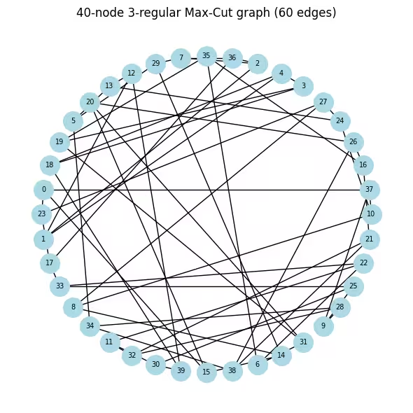
Cost operator: 40 qubits, 60 Pauli terms
c* range: [0.000, 1.000]  theta range: [1.047, 2.094] rad

Transpiled circuit: 2Q depth=86

# ── Classical baseline via simulated annealing ────────────────────
# Run SA before any hardware calls to get a strong classical reference cut
# value. SA is fast (seconds), needs no solver license, and reliably finds
# near-optimal solutions on 40-node graphs. We use sa_cut as the denominator
# for the approximation ratio instead of the looser QP upper bound.
#
# At each step we flip a random node and accept the move if it improves the
# cut, or with probability exp(delta/T) otherwise. Temperature T decays
# geometrically, allowing uphill moves early on to escape local minima.
def simulated_annealing_maxcut(
    G, seed=0, T0=2.0, T_min=1e-4, alpha=0.995, n_steps=100_000
):
    rng_sa = np.random.default_rng(seed)
    n = G.number_of_nodes()
    x = rng_sa.integers(0, 2, n)
    best_x = x.copy()
    best_cut = sum(1 for u, v in G.edges() if x[u] != x[v])
    T = T0
    for _ in range(n_steps):
        i = rng_sa.integers(0, n)
        delta = sum((-1 if x[i] != x[nb] else 1) for nb in G.neighbors(i))
        if delta > 0 or rng_sa.random() < np.exp(delta / T):
            x[i] ^= 1
            cut = sum(1 for u, v in G.edges() if x[u] != x[v])
            if cut > best_cut:
                best_cut, best_x = cut, x.copy()
        T = max(T * alpha, T_min)
    return best_x, best_cut

sa_solution, sa_cut = simulated_annealing_maxcut(G_large)
print(f"Simulated annealing cut value: {sa_cut}  (classical reference)")

# ── Step 3: Execution on hardware ───────────────────────────
# A Session reserves the backend so the COBYLA iterations and final sampling
# run back-to-back without re-queuing between jobs — important when the
# optimizer submits many short jobs sequentially. All jobs are tagged with
# "TUT_WSQAOA" for traceability in the IBM Quantum dashboard.
#
# EstimatorV2 with resilience_level=1 enables twirled readout error extinction
# (TREX), which corrects systematic measurement bit-flip errors without extra
# circuit overhead. 4096 shots per call balances estimation noise vs. job time.
estimator_options = EstimatorOptions()
estimator_options.resilience_level = 1
estimator_options.default_shots = 4096
estimator_options.environment.job_tags = ["TUT_WSQAOA"]

# Align the cost observable with the physical qubit layout chosen by the transpiler
cost_op_isa = cost_op_large.apply_layout(ws_isa_large.layout)
ws_param_order_isa = list(ws_isa_large.parameters)

ws_history_hw = []

with Session(backend=backend) as session:
    estimator_hw = Estimator(mode=session, options=estimator_options)

    def hw_cost_fn(params):
        bound = ws_isa_large.assign_parameters(
            dict(zip(ws_param_order_isa, params))
        )
        energy = (
            estimator_hw.run([(bound, cost_op_isa)]).result()[0].data.evs.real
        )
        ws_history_hw.append(float(energy))
        print(
            f"  iter {len(ws_history_hw):>3d}  <H_C> = {energy:.4f}", end="\r"
        )
        return float(energy)

    # Warm-start initialization: gamma=0 means the cost unitary is the identity on
    # the first call, so COBYLA immediately evaluates the warm-start state itself —
    # a much better starting signal than a random point.
    ws_params0_hw = np.concatenate(
        [np.zeros(p_large), np.full(p_large, np.pi / 4)]
    )

    ws_result_hw = minimize(
        hw_cost_fn,
        ws_params0_hw,
        method="COBYLA",
        options={"maxiter": 150, "rhobeg": 0.3},
    )
    print(
        f"\nOptimization complete: energy={ws_result_hw.fun:.4f}, "
        f"iterations={len(ws_history_hw)}"
    )

    # ── Step 3b: Sample the optimized circuit ──────────────────────────────────
    # Use 8192 shots for the final sample to get a reliable mode estimate.
    sampler_hw = Sampler(
        mode=session,
        options={"environment": {"job_tags": ["TUT_WSQAOA"]}},
    )
    ws_bound_hw = ws_isa_large.assign_parameters(
        dict(zip(ws_param_order_isa, ws_result_hw.x))
    )
    counts_hw = (
        sampler_hw.run([ws_bound_hw], shots=8192)
        .result()[0]
        .data.meas.get_counts()
    )

best_bs_hw = max(counts_hw, key=counts_hw.get)
best_count = counts_hw[best_bs_hw]
total_shots = sum(counts_hw.values())

# Decode: Qiskit returns bitstrings with qubit 0 at the rightmost position,
# so reversing the string maps character index i to variable x_i.
cut_val_hw, s0_hw, s1_hw = evaluate_cut(best_bs_hw[::-1], G_large)

# Compare against simulated annealing.
# A ratio >= 1.0 means WS-QAOA matched or beat the classical SA solution.
# A ratio close to 1.0 (e.g. > 0.95) shows the quantum result is competitive.
approx_ratio_hw = cut_val_hw / sa_cut
print(
    f"Most-probable bitstring frequency: {best_count}/{total_shots} "
    f"({100*best_count/total_shots:.1f}%)"
)
print(
    f"WS-QAOA cut: {cut_val_hw}  |  SA cut: {sa_cut}  "
    f"|  Approximation ratio vs SA: {approx_ratio_hw:.4f}"
)

# Visualize both solutions side-by-side on the graph.
# Blue = partition S, orange = partition S-bar.
# Edges crossing between colors are the ones counted in the cut.
fig, axes = plt.subplots(1, 2, figsize=(14, 6))
for ax, assignment, cut, title in [
    (
        axes[0],
        list(sa_solution),
        sa_cut,
        f"Simulated Annealing (cut={sa_cut})",
    ),
    (
        axes[1],
        [int(b) for b in best_bs_hw[::-1]],
        cut_val_hw,
        f"WS-QAOA hardware (cut={cut_val_hw})",
    ),
]:
    colors = [
        "skyblue" if assignment[i] == 0 else "salmon" for i in G_large.nodes()
    ]
    nx.draw(
        G_large,
        pos_large,
        with_labels=True,
        node_color=colors,
        node_size=400,
        font_size=7,
        ax=ax,
    )
    ax.set_title(title)
plt.suptitle("Max-Cut partitions: SA vs WS-QAOA", fontsize=13)
plt.tight_layout()
plt.show()

# ── Step 4: Convergence plot and summary ──────────────────────────────────
# On real hardware the trace will be noisy (shot noise + gate errors), but the
# overall downward trend confirms that COBYLA is making progress despite noise.
fig, ax = plt.subplots(figsize=(7, 4))
ax.plot(ws_history_hw, color="tab:orange", label="WS-QAOA (hardware)")
ax.axhline(
    ws_result_hw.fun,
    color="tab:orange",
    linestyle=":",
    label=f"Final energy ({ws_result_hw.fun:.3f})",
)
ax.set_xlabel("Optimizer call")
ax.set_ylabel(r"$\langle H_C \rangle$")
ax.set_title(f"WS-QAOA convergence on {backend.name} (40 qubits, p=1)")
ax.legend()
plt.tight_layout()
plt.show()

print("\n=== Large Scale Summary ===")
print(f"{'Metric':<38} {'Value':>10}")
print("-" * 50)
print(f"{'Nodes / Edges':<38} {N_LARGE:>5} / {len(edges_large):<4}")
print(f"{'QAOA layers (p)':<38} {p_large:>10}")
print(f"{'Transpiled ECR gate count':<38} {ecr_count:>10}")
print(f"{'Transpiled circuit depth':<38} {ws_isa_large.depth():>10}")
print(f"{'Optimizer iterations':<38} {len(ws_history_hw):>10}")
print(f"{'WS-QAOA energy (hardware)':<38} {ws_result_hw.fun:>10.4f}")
print(f"{'Cut value':<38} {cut_val_hw:>10}")
print(f"{'Simulated annealing cut value':<38} {sa_cut:>10}")
print(f"{'Approximation ratio (vs SA)':<38} {approx_ratio_hw:>10.4f}")

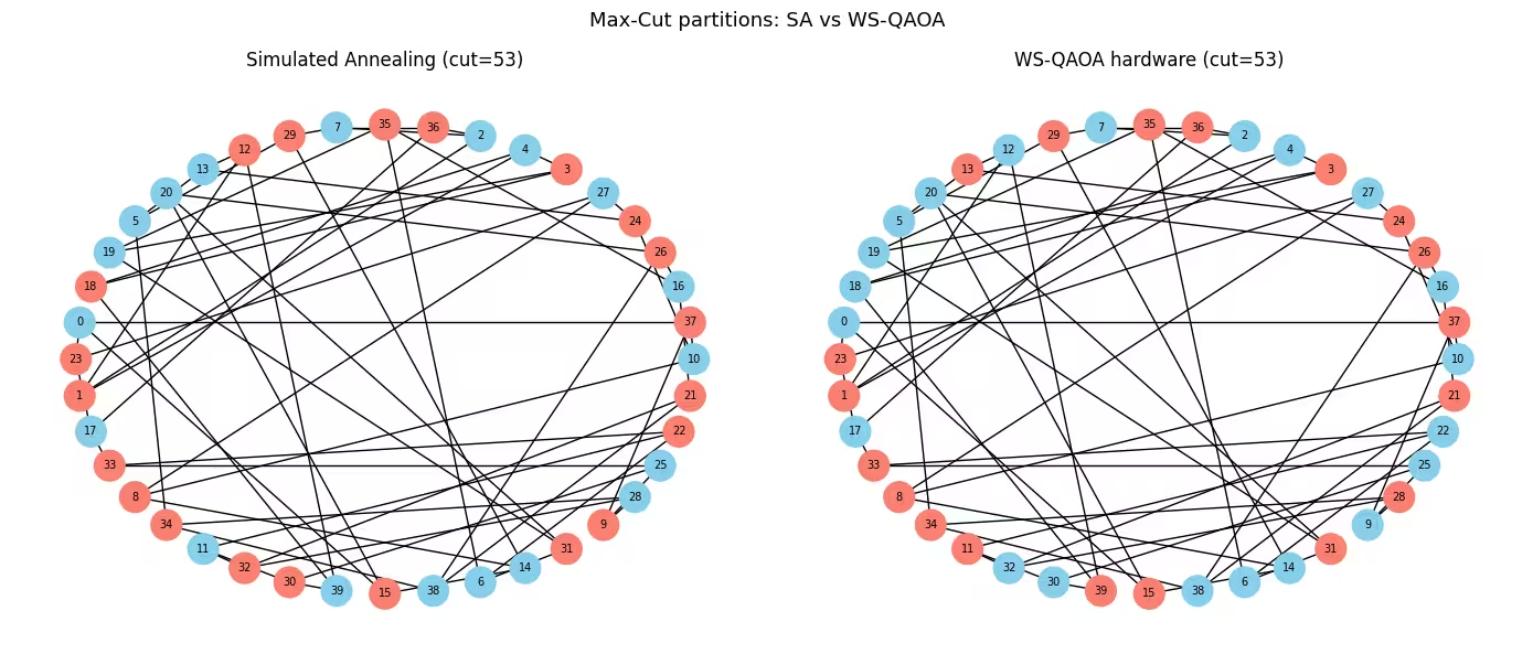
Simulated annealing cut value: 53  (classical reference)
  iter  31  <H_C> = -12.4094
Optimization complete: energy=-13.0256, iterations=31
Most-probable bitstring frequency: 4/8192 (0.0%)
WS-QAOA cut: 53  |  SA cut: 53  |  Approximation ratio vs SA: 1.0000

=== Large Scale Summary ===
Metric                                      Value
--------------------------------------------------
Nodes / Edges                             40 / 60  
QAOA layers (p)                                 1
Transpiled ECR gate count                       0
Transpiled circuit depth                      276
Optimizer iterations                           31
WS-QAOA energy (hardware)                -13.0256
Cut value                                      53
Simulated annealing cut value                  53
Approximation ratio (vs SA)                1.0000

次のステップ

推奨事項

この内容に興味を持たれた方には、以下の資料もお勧めします。

• より高いQAOAレイヤー: pを増やして、両方のアルゴリズムがより多くのCircuitレイヤーでどのように改善されるか、また低い深さでのWS-QAOAの優位性が持続するかどうかを確認してください。
• Qiskitアドオン最適化マッパー: ドキュメントを探索し、異なる組み合わせ問題のモデル化や、連続緩和のための異なるソルバーの使用を試してみてください。

参考文献

[1] D. J. Egger, J. Mareček, and S. Woerner, "Warm-starting quantum optimization," Quantum, vol. 5, p. 479, 2021. arXiv:2009.10095

[2] E. Farhi, J. Goldstone, and S. Gutmann, "A quantum approximate optimization algorithm," arXiv:1411.4028, 2014.