時間発展回路のための近似量子コンパイル
使用時間の目安:Heronプロセッサで15秒程度(注意:これは目安です。実際の実行時間は異なる場合があります。)
学習成果
このチュートリアルを完了すると、以下の情報を理解できるようになります:
- AQC-Tensor Qiskitアドオンを使用して、深いトロッター回路を浅いアンザッツ回路に圧縮する方法
- トロッター回路からパラメータ化されたアンザッツを生成し、テンソルネットワーク(MPS)手法を使用してパラメータを最適化する方法
- 圧縮された回路のターゲット発展に対する忠実度を評価し、量子ハードウェア上で実行する方法
前提条件
以下のトピックに事前に慣れておくことをお勧めします:
背景
このチュートリアルでは、テンソルネットワークを用いた近似量子コンパイル(AQC-Tensor)をQiskitで実装し、量子回路の性能を向上させる方法を示します。AQC-Tensorは、シミュレーション精度を維持しながら、深いトロッター回路をより浅いハードウェア対応の回路に圧縮します。
AQC-Tensorの仕組み
ハミルトニアン を トロッターステップを使用して合計時間 でシミュレーションする場合を考えましょう。完全なトロッター回路は次のとおりです:
回路深度を管理可能な状態に保つためにトロッターステップ数を少なくすると、大きなトロッター誤差が生じます。AQC-Tensorは精度と深度を分離することでこの緊張を解消します:
-
ターゲット回路(高精度・深い): 同じ発展時間に対してより多くのステップ(例えば )のトロッター回路を構築します。この回路はトロッター誤差がはるかに少ないですが、ハードウェアには深すぎます。行列積状態(MPS)として古典的にのみシミュレーションされるため、深度は問題になりません。
-
アンザッツ回路(低深度・パラメータ化): 1ステップのトロッター回路と同じ構造を持つパラメータ化された回路 を定義します。 となるよう初期化し、その後 が高精度のターゲット状態をできるだけ忠実に再現するよう を反復的に最適化します。
結果として、単一のトロッターステップの深度を保ちながら、多くのステップと同等の精度を達成する回路が得られます。これにより近い将来の量子ハードウェアでの実行が可能になります。
AQC-Tensorを使用すべき場面
AQC-Tensorが最も効果的な場合:
- 回路深度がハードウェアのコヒーレンス時間を超える場合。 トロッターシミュレーションがデバイスで対応できるよりも多くのトロッターステップを必要とする場合、AQC-Tensorは発展をより浅い回路に圧縮できます。
- エンタングルメントが古典的に扱いやすい場合。 時間発展した状態のエンタングルメントの総量は、主に発展時間 に依存し、トロッターステップ数 には依存しません。つまり、 ステップのターゲット回路は、 が結合次元を管理可能な状態に保つのに十分短い限り、 ステップの回路と同様にMPSとして表現するのが難しくありません。
- 自然なアンザッツが存在する場合。 アンザッツはトロッター回路の構造を反映するため、明確に定義された初期パラメータを持つ物理的に動機付けられた出発点を提供し、任意の変分アンザッツにありがちな収束問題を回避できます。
このアプローチは一般的な回路圧縮とは異なります:任意のユニタリをより少ないゲートで近似しようとするのではなく、AQC-Tensorは同じゲート構造を保ちながらパラメータを最適化してトロッター誤差を削減します。詳細については、AQC-Tensorのドキュメントを参照してください。
このチュートリアルでは、完全な状態準備AQC-Tensorワークフローを案内します:ハミルトニアンの定義、トロッター回路の生成、テンソルネットワーク最適化による圧縮、そしてIBM Quantum®ハードウェアでの実行結果の処理を行います。
要件
このチュートリアルを始める前に、以下がインストールされていることを確認してください:
- Qiskit SDK v2.0以降(可視化サポート付き)
- Qiskit Runtime v0.22以降(
pip install qiskit-ibm-runtime) - AQC-Tensor Qiskitアドオン(
pip install 'qiskit-addon-aqc-tensor[aer,quimb-jax]')
セットアップ
# Added by doQumentation — required packages for this notebook
!pip install -q matplotlib numpy qiskit qiskit-addon-aqc-tensor qiskit-addon-utils qiskit-ibm-runtime quimb rustworkx scipy
import numpy as np
import quimb.tensor
import datetime
import matplotlib.pyplot as plt

from scipy.linalg import expm
from scipy.optimize import OptimizeResult, minimize

from qiskit.quantum_info import SparsePauliOp, Pauli
from qiskit.transpiler import CouplingMap
from qiskit.transpiler.preset_passmanagers import generate_preset_pass_manager
from qiskit import QuantumCircuit
from qiskit.synthesis import SuzukiTrotter

from qiskit_addon_utils.problem_generators import (
    generate_time_evolution_circuit,
)
from qiskit_addon_aqc_tensor.ansatz_generation import (
    generate_ansatz_from_circuit,
)
from qiskit_addon_aqc_tensor.objective import MaximizeStateFidelity
from qiskit_addon_aqc_tensor.simulation.quimb import QuimbSimulator
from qiskit_addon_aqc_tensor.simulation import tensornetwork_from_circuit
from qiskit_addon_aqc_tensor.simulation import compute_overlap

from qiskit_ibm_runtime import QiskitRuntimeService
from qiskit_ibm_runtime import EstimatorV2 as Estimator
from qiskit_ibm_runtime.fake_provider import FakeKyiv

from rustworkx.visualization import graphviz_draw
小規模シミュレータの例
このセクションでは、10サイトのシステムを使用してAQC-Tensorワークフローのステップを順に説明します。スピン相互作用と磁性特性の研究において広く研究されている10サイトXXZスピン鎖のダイナミクスをシミュレーションします。
ハミルトニアンは次のとおりです:
ここで、は辺のランダム係数であり、です。
ステップ1:古典的な入力を量子問題にマッピング
このステップでは以下を行います:
- ハミルトニアン、オブザーバブル、初期状態を定義します。
- 後の比較のために期待値を古典的に正確に計算します。
- 高精度のトロッター回路(AQCターゲット)を生成し、AQC-Tensorを使用して低深度のアンザッツに圧縮します。
ハミルトニアン・オブザーバブル・初期状態の設定
# L is the number of sites in the 1D spin chain
L = 10

# Generate the coupling map
edge_list = [(i - 1, i) for i in range(1, L)]
even_edges = edge_list[::2]
odd_edges = edge_list[1::2]
coupling_map = CouplingMap(edge_list)

# Generate random coefficients for our XXZ Hamiltonian
np.random.seed(0)
Js = np.random.rand(L - 1) + 0.5 * np.ones(L - 1)
hamiltonian = SparsePauliOp(Pauli("I" * L))
for i, edge in enumerate(even_edges + odd_edges):
    hamiltonian += SparsePauliOp.from_sparse_list(
        [
            ("XX", (edge), Js[i] / 2),
            ("YY", (edge), Js[i] / 2),
            ("ZZ", (edge), Js[i]),
        ],
        num_qubits=L,
    )

# Generate a ZZ observable between the two middle qubits
observable = SparsePauliOp.from_sparse_list(
    [("ZZ", (L // 2 - 1, L // 2), 1.0)], num_qubits=L
)

# Generate an initial Néel state |1010101010⟩
initial_state_circuit = QuantumCircuit(L)
for i in range(L):
    if i % 2:
        initial_state_circuit.x(i)

print("Hamiltonian:", hamiltonian)
print("Observable:", observable)
graphviz_draw(coupling_map.graph, method="circo")
Hamiltonian: SparsePauliOp(['IIIIIIIIII', 'IIIIIIIIXX', 'IIIIIIIIYY', 'IIIIIIIIZZ', 'IIIIIIXXII', 'IIIIIIYYII', 'IIIIIIZZII', 'IIIIXXIIII', 'IIIIYYIIII', 'IIIIZZIIII', 'IIXXIIIIII', 'IIYYIIIIII', 'IIZZIIIIII', 'XXIIIIIIII', 'YYIIIIIIII', 'ZZIIIIIIII', 'IIIIIIIXXI', 'IIIIIIIYYI', 'IIIIIIIZZI', 'IIIIIXXIII', 'IIIIIYYIII', 'IIIIIZZIII', 'IIIXXIIIII', 'IIIYYIIIII', 'IIIZZIIIII', 'IXXIIIIIII', 'IYYIIIIIII', 'IZZIIIIIII'],
              coeffs=[1.        +0.j, 0.52440675+0.j, 0.52440675+0.j, 1.0488135 +0.j,
 0.60759468+0.j, 0.60759468+0.j, 1.21518937+0.j, 0.55138169+0.j,
 0.55138169+0.j, 1.10276338+0.j, 0.52244159+0.j, 0.52244159+0.j,
 1.04488318+0.j, 0.4618274 +0.j, 0.4618274 +0.j, 0.9236548 +0.j,
 0.57294706+0.j, 0.57294706+0.j, 1.14589411+0.j, 0.46879361+0.j,
 0.46879361+0.j, 0.93758721+0.j, 0.6958865 +0.j, 0.6958865 +0.j,
 1.391773  +0.j, 0.73183138+0.j, 0.73183138+0.j, 1.46366276+0.j])
Observable: SparsePauliOp(['IIIIZZIIII'],
              coeffs=[1.+0.j])

正確な期待値の計算
このサイズのシステムでは、行列の指数化を使用して時間発展後の期待値を直接計算できます。これにより、AQC回路の精度を評価するための真の基準値が得られます。
aqc_evolution_time = 0.2

# Each baseline Trotter step covers dt = aqc_evolution_time / 3
# The subsequent (uncompressed) step covers 1 additional dt
subsequent_evolution_time = aqc_evolution_time / 3
total_evolution_time = aqc_evolution_time + subsequent_evolution_time

# Compute exact expectation value via matrix exponentiation
H_matrix = hamiltonian.to_matrix()
U_exact = expm(-1j * H_matrix * total_evolution_time)

# Build the initial state vector (Néel state)
initial_state_vec = np.zeros(2**L)
state_idx = sum(2**i for i in range(L) if i % 2)
initial_state_vec[state_idx] = 1.0

# Evolve and compute expectation value
evolved_state = U_exact @ initial_state_vec
obs_matrix = observable.to_matrix()
exact_expval = (evolved_state.conj() @ obs_matrix @ evolved_state).real

print(f"AQC evolution time: {aqc_evolution_time}")
print(f"Subsequent evolution time: {subsequent_evolution_time:.6f}")
print(f"Total evolution time: {total_evolution_time:.6f}")
print(f"Exact expectation value: {exact_expval:.6f}")
AQC evolution time: 0.2
Subsequent evolution time: 0.066667
Total evolution time: 0.266667
Exact expectation value: -0.700899
AQCターゲット回路の生成
次に、ACQターゲットとして機能するトロッター回路を構築します。この回路は高精度のために多くのトロッターステップ(32)を使用します。MPSとして古典的にのみシミュレーションされ、ハードウェア上では実行されないため、大きな深度は問題になりません。
aqc_target_num_trotter_steps = 32

aqc_target_circuit = initial_state_circuit.copy()
aqc_target_circuit.compose(
    generate_time_evolution_circuit(
        hamiltonian,
        synthesis=SuzukiTrotter(reps=aqc_target_num_trotter_steps),
        time=aqc_evolution_time,
    ),
    inplace=True,
)
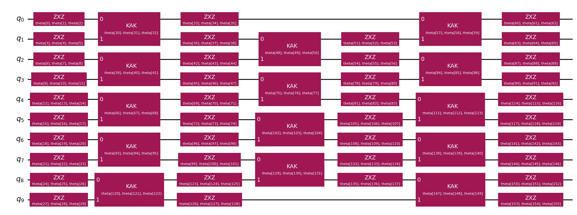
アンザッツ・初期パラメータ・後続回路・ベースライン回路の生成
次に、AQCターゲットと同じ発展時間でトロッターステップが1つだけの「良い」回路を構築します。この回路をgenerate_ansatz_from_circuitに渡すと、以下が返されます:
- 同じ2量子ビット接続性を持つ一般的なパラメータ化されたアンザッツ回路。
- アンザッツに代入すると入力回路を再現する初期パラメータ。
また、以下も構築します:
- AQC最適化部分の後に追加する(非圧縮の)1トロッターステップからなる後続回路。AQC-Tensorの初期状態チュートリアルのアプローチに従います。
- AQCなしでハードウェアで実行する場合の比較として機能する、全発展時間(
aqc_evolution_time + subsequent_evolution_time)にわたる4トロッターステップのベースライントロッター回路。AQCアンザッツ(圧縮3ステップ+非圧縮1ステップ)は、より低い深度でより高い精度を達成します。
aqc_ansatz_num_trotter_steps = 1

aqc_good_circuit = initial_state_circuit.copy()
aqc_good_circuit.compose(
    generate_time_evolution_circuit(
        hamiltonian,
        synthesis=SuzukiTrotter(reps=aqc_ansatz_num_trotter_steps),
        time=aqc_evolution_time,
    ),
    inplace=True,
)

aqc_ansatz, aqc_initial_parameters = generate_ansatz_from_circuit(
    aqc_good_circuit
)

# Subsequent circuit: 1 non-compressed Trotter step appended after AQC
subsequent_num_trotter_steps = 1
subsequent_circuit = generate_time_evolution_circuit(
    hamiltonian,
    synthesis=SuzukiTrotter(reps=subsequent_num_trotter_steps),
    time=subsequent_evolution_time,
)

# Baseline Trotter circuit: 4 Trotter steps over total evolution time, no AQC
baseline_num_trotter_steps = 4
baseline_circuit = initial_state_circuit.copy()
baseline_circuit.compose(
    generate_time_evolution_circuit(
        hamiltonian,
        synthesis=SuzukiTrotter(reps=baseline_num_trotter_steps),
        time=total_evolution_time,
    ),
    inplace=True,
)

print(
    f"Target circuit:      depth {aqc_target_circuit.depth(lambda x: x.operation.num_qubits == 2)}"
)
print(
    f"Baseline circuit:    depth {baseline_circuit.depth(lambda x: x.operation.num_qubits == 2)} ({baseline_num_trotter_steps} Trotter steps, time={total_evolution_time:.4f})"
)
print(
    f"Subsequent circuit:  depth {subsequent_circuit.depth(lambda x: x.operation.num_qubits == 2)} ({subsequent_num_trotter_steps} Trotter step, time={subsequent_evolution_time:.4f})"
)
print(
    f"Ansatz circuit:      depth {aqc_ansatz.depth(lambda x: x.operation.num_qubits == 2)}, with {len(aqc_initial_parameters)} parameters"
)
aqc_ansatz.draw("mpl", fold=-1)
Target circuit:      depth 384
Baseline circuit:    depth 48 (4 Trotter steps, time=0.2667)
Subsequent circuit:  depth 12 (1 Trotter step, time=0.0667)
Ansatz circuit:      depth 3, with 156 parameters
テンソルネットワークシミュレーションの設定とターゲットMPSの構築
勾配ベースの最適化の自動微分にJAXを使用したquimb行列積状態(MPS)回路シミュレータを使用します。次に、ターゲット状態のMPS表現を構築し、初期アンザッツとターゲットの間の初期忠実度を評価します。この問題インスタンスは比較的小規模な例であるため、初期忠実度はかなり高い値から始まります。
simulator_settings = QuimbSimulator(
    quimb.tensor.CircuitMPS, autodiff_backend="jax"
)

aqc_target_mps = tensornetwork_from_circuit(
    aqc_target_circuit, simulator_settings
)
print("Target MPS maximum bond dimension:", aqc_target_mps.psi.max_bond())

good_mps = tensornetwork_from_circuit(aqc_good_circuit, simulator_settings)
starting_fidelity = abs(compute_overlap(good_mps, aqc_target_mps)) ** 2
print(f"Starting fidelity: {starting_fidelity:.6f}")
Target MPS maximum bond dimension: 5
Starting fidelity: 0.998246
アンザッツパラメータの最適化
MaximizeStateFidelityコスト関数をL-BFGS-Bオプティマイザを使用して最小化します。オプティマイザはアンザッツパラメータを反復的に調整して、アンザッツ回路とターゲットMPSの間の忠実度を最大化します。
aqc_stopping_fidelity = 1
aqc_max_iterations = 500

stopping_point = 1.0 - aqc_stopping_fidelity
objective = MaximizeStateFidelity(
    aqc_target_mps, aqc_ansatz, simulator_settings
)

def callback(intermediate_result: OptimizeResult):
    fidelity = 1 - intermediate_result.fun
    print(
        f"{datetime.datetime.now()} Intermediate result: Fidelity {fidelity:.8f}"
    )
    if intermediate_result.fun < stopping_point:
        raise StopIteration

result = minimize(
    objective,
    aqc_initial_parameters,
    method="L-BFGS-B",
    jac=True,
    options={"maxiter": aqc_max_iterations},
    callback=callback,
)
if result.status not in (0, 1, 99):
    raise RuntimeError(
        f"Optimization failed: {result.message} (status={result.status})"
    )

print(f"Done after {result.nit} iterations.")
aqc_final_parameters = result.x
2026-05-18 13:14:49.731596 Intermediate result: Fidelity 0.99952882
2026-05-18 13:14:49.734425 Intermediate result: Fidelity 0.99958531
2026-05-18 13:14:49.737101 Intermediate result: Fidelity 0.99960093
2026-05-18 13:14:49.739813 Intermediate result: Fidelity 0.99961046
2026-05-18 13:14:49.742969 Intermediate result: Fidelity 0.99962560
2026-05-18 13:14:49.745916 Intermediate result: Fidelity 0.99964395
2026-05-18 13:14:49.748615 Intermediate result: Fidelity 0.99968150
2026-05-18 13:14:49.753684 Intermediate result: Fidelity 0.99970569
2026-05-18 13:14:49.756208 Intermediate result: Fidelity 0.99973788
2026-05-18 13:14:49.759067 Intermediate result: Fidelity 0.99975385
2026-05-18 13:14:49.762321 Intermediate result: Fidelity 0.99976458
2026-05-18 13:14:49.765526 Intermediate result: Fidelity 0.99977661
2026-05-18 13:14:49.768496 Intermediate result: Fidelity 0.99978663
2026-05-18 13:14:49.771278 Intermediate result: Fidelity 0.99980236
2026-05-18 13:14:49.773735 Intermediate result: Fidelity 0.99981607
2026-05-18 13:14:49.776339 Intermediate result: Fidelity 0.99982811
2026-05-18 13:14:49.779177 Intermediate result: Fidelity 0.99985827
2026-05-18 13:14:49.782243 Intermediate result: Fidelity 0.99988354
2026-05-18 13:14:49.784904 Intermediate result: Fidelity 0.99991608
2026-05-18 13:14:49.787737 Intermediate result: Fidelity 0.99993336
2026-05-18 13:14:49.790414 Intermediate result: Fidelity 0.99993956
2026-05-18 13:14:49.793029 Intermediate result: Fidelity 0.99994421
2026-05-18 13:14:49.795585 Intermediate result: Fidelity 0.99994743
2026-05-18 13:14:49.835045 Intermediate result: Fidelity 0.99994791
2026-05-18 13:14:49.839786 Intermediate result: Fidelity 0.99994803
2026-05-18 13:14:49.842403 Intermediate result: Fidelity 0.99994898
2026-05-18 13:14:49.873779 Intermediate result: Fidelity 0.99994898
Done after 27 iterations.
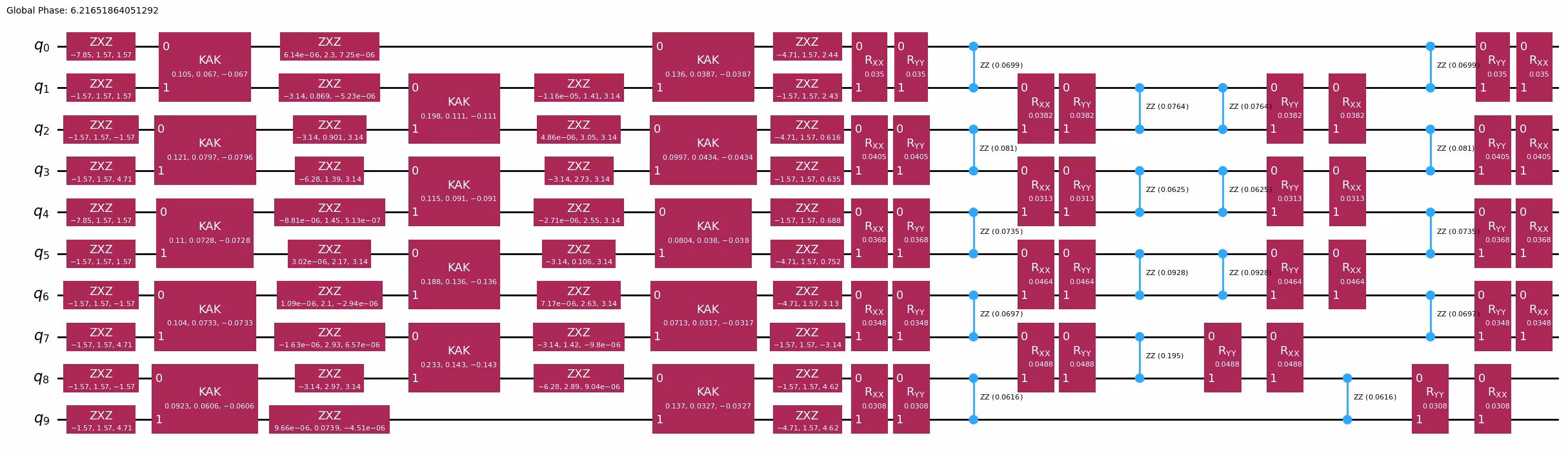
最終AQC回路の組み立て
最適化されたパラメータをアンザッツに代入し、後続の(非圧縮)トロッターステップを追加します。得られた回路の深度は、圧縮された1ステップ分と非圧縮の1ステップ分を合わせた深度ですが、圧縮部分は32トロッターステップの精度を近似しています。
aqc_final_circuit = aqc_ansatz.assign_parameters(aqc_final_parameters)
aqc_final_circuit.compose(subsequent_circuit, inplace=True)
aqc_final_circuit.draw("mpl", fold=-1)
ステップ 2: 量子ハードウェア実行のための問題の最適化
この小規模な例では、フェイクバックエンド(FakeKyiv)を使用してハードウェア実行をローカルでシミュレーションします。AQC最適化された回路(aqc_final_circuit)とベースライントロッター回路(baseline_circuit:AQCなしの全発展時間にわたる4トロッターステップ)の両方を、optimization_level=3 を指定してバックエンドの命令セットアーキテクチャ(ISA)にトランスパイルし、さらに回路深度を削減します。
backend = FakeKyiv()

pass_manager = generate_preset_pass_manager(
    backend=backend, optimization_level=3
)

# Transpile the AQC-optimized circuit (compressed + subsequent step)
isa_circuit = pass_manager.run(aqc_final_circuit)
isa_observable = observable.apply_layout(isa_circuit.layout)
print(
    "AQC circuit depth:",
    isa_circuit.depth(lambda x: x.operation.num_qubits == 2),
)

# Transpile the baseline Trotter circuit (no AQC optimization)
isa_baseline_circuit = pass_manager.run(baseline_circuit)
isa_baseline_observable = observable.apply_layout(isa_baseline_circuit.layout)
print(
    "Baseline Trotter circuit depth:",
    isa_baseline_circuit.depth(lambda x: x.operation.num_qubits == 2),
)
AQC circuit depth: 15
Baseline Trotter circuit depth: 27
ステップ 3: Qiskit プリミティブを使用した実行
フェイクバックエンドで EstimatorV2 プリミティブを使用し、AQC最適化された回路とベースライントロッター回路の両方を実行して、それぞれのZZオブザーバブルを測定します。
estimator = Estimator(backend)

# Run both circuits
aqc_result = estimator.run([(isa_circuit, isa_observable)]).result()
baseline_result = estimator.run(
    [(isa_baseline_circuit, isa_baseline_observable)]
).result()
ステップ 4: 後処理と所望の古典形式での結果の返却
両方の実行から期待値を抽出し、正確な結果と比較します。ベースライントロッター回路は、同じ回路深度でAQCなしの場合に得られる結果を示し、AQC回路はテンソルネットワーク最適化による改善を示します。
aqc_expval = aqc_result[0].data.evs.tolist()
baseline_expval = baseline_result[0].data.evs.tolist()

print(f"Exact:              {exact_expval:.4f}")
print(
    f"Baseline Trotter:   {baseline_expval:.4f}, |\u0394| = {np.abs(exact_expval - baseline_expval):.4f}  (depth {isa_baseline_circuit.depth(lambda x: x.operation.num_qubits == 2)}, {baseline_num_trotter_steps} steps)"
)
print(
    f"AQC (3+1):          {aqc_expval:.4f}, |\u0394| = {np.abs(exact_expval - aqc_expval):.4f}  (depth {isa_circuit.depth(lambda x: x.operation.num_qubits == 2)}, compressed+subsequent)"
)
Exact:              -0.7009
Baseline Trotter:   -0.5400, |Δ| = 0.1609  (depth 27, 4 steps)
AQC (3+1):          -0.5728, |Δ| = 0.1281  (depth 15, compressed+subsequent)
plt.style.use("seaborn-v0_8")

labels = [
    f"Baseline Trotter\n({baseline_num_trotter_steps} steps, depth {isa_baseline_circuit.depth(lambda x: x.operation.num_qubits == 2)})",
    f"AQC (3+1)\n(depth {isa_circuit.depth(lambda x: x.operation.num_qubits == 2)})",
]
values = [baseline_expval, aqc_expval]
colors = ["tab:orange", "tab:blue"]

plt.figure(figsize=(8, 5))
bars = plt.bar(labels, values, color=colors, width=0.5)
plt.axhline(
    y=exact_expval,
    color="tab:green",
    linestyle="--",
    linewidth=2,
    label=f"Exact ({exact_expval:.4f})",
)
plt.ylabel("Expected Value")
plt.title(
    "AQC-Tensor (3 compressed + 1 uncompressed) vs Baseline Trotter (10-site XXZ)"
)
plt.legend()
for bar in bars:
    y_val = bar.get_height()
    plt.text(
        bar.get_x() + bar.get_width() / 2.0,
        y_val,
        f"{y_val:.4f}",
        ha="center",
        va="bottom" if y_val >= 0 else "top",
    )
plt.axhline(y=0, color="black", linewidth=0.3)
plt.tight_layout()
plt.show()

大規模なハードウェアの例
ここでは、50サイト XXZ モデルにスケールアップして、より現実的な問題サイズで AQC-Tensor を示します。ワークフローは小規模の例と同じです:3つのトロッターステップを AQC で圧縮し、1つの非圧縮ステップを追加します。
このサイズのシステムでは行列の指数化は実行不可能( 次元)なため、完全な時間にわたって発展させた高精度 MPS から参照期待値を直接計算します。
ステップ 1〜4 を統合
# -------------------------Step 1-------------------------

# Define the 50-site spin chain
L = 50
edge_list = [(i - 1, i) for i in range(1, L)]
even_edges = edge_list[::2]
odd_edges = edge_list[1::2]
coupling_map = CouplingMap(edge_list)

# Random XXZ Hamiltonian
np.random.seed(0)
Js = np.random.rand(L - 1) + 0.5 * np.ones(L - 1)
hamiltonian = SparsePauliOp(Pauli("I" * L))
for i, edge in enumerate(even_edges + odd_edges):
    hamiltonian += SparsePauliOp.from_sparse_list(
        [
            ("XX", (edge), Js[i] / 2),
            ("YY", (edge), Js[i] / 2),
            ("ZZ", (edge), Js[i]),
        ],
        num_qubits=L,
    )

observable = SparsePauliOp.from_sparse_list(
    [("ZZ", (L // 2 - 1, L // 2), 1.0)], num_qubits=L
)

# Initial Néel state
initial_state_circuit = QuantumCircuit(L)
for i in range(L):
    if i % 2:
        initial_state_circuit.x(i)

# Time parameters
aqc_evolution_time = 0.2
subsequent_evolution_time = aqc_evolution_time / 3
total_evolution_time = aqc_evolution_time + subsequent_evolution_time

# AQC target circuit (high-accuracy, 32 Trotter steps for AQC portion)
aqc_target_num_trotter_steps = 32

aqc_target_circuit = initial_state_circuit.copy()
aqc_target_circuit.compose(
    generate_time_evolution_circuit(
        hamiltonian,
        synthesis=SuzukiTrotter(reps=aqc_target_num_trotter_steps),
        time=aqc_evolution_time,
    ),
    inplace=True,
)

# Generate ansatz from 1-step Trotter circuit
aqc_good_circuit = initial_state_circuit.copy()
aqc_good_circuit.compose(
    generate_time_evolution_circuit(
        hamiltonian,
        synthesis=SuzukiTrotter(reps=1),
        time=aqc_evolution_time,
    ),
    inplace=True,
)

aqc_ansatz, aqc_initial_parameters = generate_ansatz_from_circuit(
    aqc_good_circuit
)

# Subsequent circuit: 1 non-compressed Trotter step
subsequent_circuit = generate_time_evolution_circuit(
    hamiltonian,
    synthesis=SuzukiTrotter(reps=1),
    time=subsequent_evolution_time,
)

# Baseline Trotter circuit: 4 Trotter steps over total evolution time, no AQC
baseline_num_trotter_steps = 4
baseline_circuit = initial_state_circuit.copy()
baseline_circuit.compose(
    generate_time_evolution_circuit(
        hamiltonian,
        synthesis=SuzukiTrotter(reps=baseline_num_trotter_steps),
        time=total_evolution_time,
    ),
    inplace=True,
)
print(
    f"Target circuit:  depth {aqc_target_circuit.depth(lambda x: x.operation.num_qubits == 2)}"
)
print(
    f"Ansatz circuit:  depth {aqc_ansatz.depth(lambda x: x.operation.num_qubits == 2)}, with {len(aqc_initial_parameters)} parameters"
)
print(
    f"Subsequent circuit: depth {subsequent_circuit.depth(lambda x: x.operation.num_qubits == 2)}"
)
print(
    f"Baseline circuit:   depth {baseline_circuit.depth(lambda x: x.operation.num_qubits == 2)} ({baseline_num_trotter_steps} steps, time={total_evolution_time:.4f})"
)

# Build target MPS and compute reference expectation value
simulator_settings = QuimbSimulator(
    quimb.tensor.CircuitMPS, autodiff_backend="jax"
)
aqc_target_mps = tensornetwork_from_circuit(
    aqc_target_circuit, simulator_settings
)
print("Target MPS maximum bond dimension:", aqc_target_mps.psi.max_bond())

# For the reference expectation value, we need the full evolution (AQC + subsequent)
# Build a high-accuracy full circuit for MPS reference
full_target_circuit = initial_state_circuit.copy()
full_target_circuit.compose(
    generate_time_evolution_circuit(
        hamiltonian,
        synthesis=SuzukiTrotter(reps=aqc_target_num_trotter_steps),
        time=total_evolution_time,
    ),
    inplace=True,
)
full_target_mps = tensornetwork_from_circuit(
    full_target_circuit, simulator_settings
)
exact_expval = full_target_mps.local_expectation(
    quimb.pauli("Z") & quimb.pauli("Z"), (L // 2 - 1, L // 2)
).real.item()
print(f"Reference expectation value (from MPS): {exact_expval:.6f}")

# Optimize ansatz parameters
objective = MaximizeStateFidelity(
    aqc_target_mps, aqc_ansatz, simulator_settings
)

def callback(intermediate_result: OptimizeResult):
    fidelity = 1 - intermediate_result.fun
    print(
        f"{datetime.datetime.now()} Intermediate result: Fidelity {fidelity:.8f}"
    )

result = minimize(
    objective,
    aqc_initial_parameters,
    method="L-BFGS-B",
    jac=True,
    options={"maxiter": 500},
    callback=callback,
)
if result.status not in (0, 1, 99):
    raise RuntimeError(
        f"Optimization failed: {result.message} (status={result.status})"
    )
print(f"Done after {result.nit} iterations.")

# Assemble the final AQC circuit: optimized ansatz + subsequent Trotter step
aqc_final_circuit = aqc_ansatz.assign_parameters(result.x)
aqc_final_circuit.compose(subsequent_circuit, inplace=True)

# -------------------------Step 2-------------------------

service = QiskitRuntimeService()
backend = service.least_busy(min_num_qubits=127)
print(backend)

pass_manager = generate_preset_pass_manager(
    backend=backend, optimization_level=3
)
isa_circuit = pass_manager.run(aqc_final_circuit)
isa_observable = observable.apply_layout(isa_circuit.layout)
print(
    "AQC circuit depth:",
    isa_circuit.depth(lambda x: x.operation.num_qubits == 2),
)

# Also transpile the baseline Trotter circuit (4 Trotter steps, no AQC)
isa_baseline_circuit = pass_manager.run(baseline_circuit)
isa_baseline_observable = observable.apply_layout(isa_baseline_circuit.layout)
print(
    "Baseline Trotter circuit depth:",
    isa_baseline_circuit.depth(lambda x: x.operation.num_qubits == 2),
)

# -------------------------Step 3-------------------------

# Submit both circuits in a single job
estimator = Estimator(backend)
estimator.options.environment.job_tags = ["TUT_AQCTE"]

job = estimator.run(
    [
        (isa_circuit, isa_observable),
        (isa_baseline_circuit, isa_baseline_observable),
    ]
)
print("Job ID:", job.job_id())
Target circuit:  depth 385
Ansatz circuit:  depth 7, with 816 parameters
Subsequent circuit: depth 12
Baseline circuit:   depth 49 (4 steps, time=0.2667)
Target MPS maximum bond dimension: 5
Reference expectation value (from MPS): -0.738669
2026-05-18 13:02:11.219150 Intermediate result: Fidelity 0.99795732
2026-05-18 13:02:11.232256 Intermediate result: Fidelity 0.99822481
2026-05-18 13:02:11.245160 Intermediate result: Fidelity 0.99829520
2026-05-18 13:02:11.257765 Intermediate result: Fidelity 0.99832379
2026-05-18 13:02:11.270280 Intermediate result: Fidelity 0.99836416
2026-05-18 13:02:11.284116 Intermediate result: Fidelity 0.99840073
2026-05-18 13:02:11.296856 Intermediate result: Fidelity 0.99846863
2026-05-18 13:02:11.309602 Intermediate result: Fidelity 0.99865244
2026-05-18 13:02:11.322012 Intermediate result: Fidelity 0.99872665
2026-05-18 13:02:11.334195 Intermediate result: Fidelity 0.99892335
2026-05-18 13:02:11.346570 Intermediate result: Fidelity 0.99901045
2026-05-18 13:02:11.359202 Intermediate result: Fidelity 0.99907181
2026-05-18 13:02:11.371511 Intermediate result: Fidelity 0.99911125
2026-05-18 13:02:11.383870 Intermediate result: Fidelity 0.99918585
2026-05-18 13:02:11.396184 Intermediate result: Fidelity 0.99921504
2026-05-18 13:02:11.408543 Intermediate result: Fidelity 0.99924936
2026-05-18 13:02:11.422557 Intermediate result: Fidelity 0.99929226
2026-05-18 13:02:11.436275 Intermediate result: Fidelity 0.99933099
2026-05-18 13:02:11.449511 Intermediate result: Fidelity 0.99935792
2026-05-18 13:02:11.462093 Intermediate result: Fidelity 0.99937925
2026-05-18 13:02:11.475783 Intermediate result: Fidelity 0.99940690
2026-05-18 13:02:11.490254 Intermediate result: Fidelity 0.99944409
2026-05-18 13:02:11.503292 Intermediate result: Fidelity 0.99946840
2026-05-18 13:02:11.516064 Intermediate result: Fidelity 0.99949378
2026-05-18 13:02:11.532861 Intermediate result: Fidelity 0.99951380
2026-05-18 13:02:11.546182 Intermediate result: Fidelity 0.99955313
2026-05-18 13:02:11.559168 Intermediate result: Fidelity 0.99955707
2026-05-18 13:02:11.571753 Intermediate result: Fidelity 0.99959306
2026-05-18 13:02:11.584257 Intermediate result: Fidelity 0.99960486
2026-05-18 13:02:11.597610 Intermediate result: Fidelity 0.99961714
2026-05-18 13:02:11.610106 Intermediate result: Fidelity 0.99962953
2026-05-18 13:02:11.622515 Intermediate result: Fidelity 0.99963525
2026-05-18 13:02:11.635543 Intermediate result: Fidelity 0.99964658
2026-05-18 13:02:11.649044 Intermediate result: Fidelity 0.99965027
2026-05-18 13:02:11.664148 Intermediate result: Fidelity 0.99965802
2026-05-18 13:02:11.678033 Intermediate result: Fidelity 0.99966731
2026-05-18 13:02:11.692714 Intermediate result: Fidelity 0.99967780
2026-05-18 13:02:11.706753 Intermediate result: Fidelity 0.99968567
2026-05-18 13:02:11.720780 Intermediate result: Fidelity 0.99969139
2026-05-18 13:02:11.733471 Intermediate result: Fidelity 0.99969628
2026-05-18 13:02:11.745998 Intermediate result: Fidelity 0.99970331
2026-05-18 13:02:11.758424 Intermediate result: Fidelity 0.99970796
2026-05-18 13:02:11.771986 Intermediate result: Fidelity 0.99971165
2026-05-18 13:02:11.785841 Intermediate result: Fidelity 0.99971892
2026-05-18 13:02:11.799105 Intermediate result: Fidelity 0.99972226
2026-05-18 13:02:11.811623 Intermediate result: Fidelity 0.99972441
2026-05-18 13:02:11.824114 Intermediate result: Fidelity 0.99972679
2026-05-18 13:02:11.837179 Intermediate result: Fidelity 0.99972965
2026-05-18 13:02:12.345479 Intermediate result: Fidelity 0.99972965
Done after 49 iterations.
<IBMBackend('ibm_pittsburgh')>
AQC circuit depth: 71
Baseline Trotter circuit depth: 111
Job ID: d85kc6o0bvlc73d5nhn0
# -------------------------Step 4-------------------------

hw_results = job.result()
aqc_expval = hw_results[0].data.evs.tolist()
baseline_expval = hw_results[1].data.evs.tolist()

print(f"Exact (MPS):        {exact_expval:.4f}")
print(
    f"Baseline Trotter:   {baseline_expval:.4f}, |\u0394| = {np.abs(exact_expval - baseline_expval):.4f}"
)
print(
    f"AQC (3+1):          {aqc_expval:.4f}, |\u0394| = {np.abs(exact_expval - aqc_expval):.4f}"
)

labels = [
    f"Baseline Trotter\n({baseline_num_trotter_steps} steps, depth {isa_baseline_circuit.depth(lambda x: x.operation.num_qubits == 2)})",
    f"AQC (3+1)\n(depth {isa_circuit.depth(lambda x: x.operation.num_qubits == 2)})",
]
values = [baseline_expval, aqc_expval]
colors = ["tab:orange", "tab:blue"]

plt.figure(figsize=(8, 5))
bars = plt.bar(labels, values, color=colors, width=0.5)
plt.axhline(
    y=exact_expval,
    color="tab:green",
    linestyle="--",
    linewidth=2,
    label=f"Exact ({exact_expval:.4f})",
)
plt.ylabel("Expected Value")
plt.title(
    "AQC-Tensor (3 compressed + 1 uncompressed) vs Baseline Trotter (50-site XXZ)"
)
plt.legend()
for bar in bars:
    y_val = bar.get_height()
    plt.text(
        bar.get_x() + bar.get_width() / 2.0,
        y_val,
        f"{y_val:.4f}",
        ha="center",
        va="bottom" if y_val >= 0 else "top",
    )
plt.axhline(y=0, color="black", linewidth=0.3)
plt.tight_layout()
plt.show()
Exact (MPS):        -0.7387
Baseline Trotter:   -0.5955, |Δ| = 0.1432
AQC (3+1):          -0.6734, |Δ| = 0.0653

次のステップ
この内容が興味深いと感じた場合は、以下の資料も参考にしてください:
- AQC-Tensor アドオンのドキュメント — 準備された状態ではなくターゲットユニタリ演算子を近似するパラメータ化された回路を最適化する関連技術であるユニタリ AQC も含まれています
- エラー緩和と抑制の技術
- エラー緩和技術の組み合わせ