トランスパイラー設定の比較

Package versions

このページのコードは以下の要件を使用して開発されました。 これらのバージョン以降を使用することを推奨します。

qiskit[all]~=2.4.0
qiskit-ibm-runtime~=0.46.1

異なるトランスパイラー設定は、古典処理時間が長くなる代わりに、回路にさまざまな最適化を提供します。このガイドでは、各種設定のパフォーマンスをテストするために、回路の作成・トランスパイル・送信の全プロセスを順を追って説明します。

同じ設定でも、ある回路の結果を改善する一方で別の回路を悪化させる場合があることに注意してください。実際のハードウェアで実行する前に、トランスパイル後の回路を必ず確認してください。

セットアップとサンプル回路の作成

# Added by doQumentation — required packages for this notebook
!pip install -q qiskit qiskit-ibm-runtime

# Create circuit to test transpiler on
from qiskit import QuantumCircuit
from qiskit.transpiler.preset_passmanagers import generate_preset_pass_manager
from qiskit.circuit.library import grover_operator, DiagonalGate

# Use Statevector object to calculate the ideal output
from qiskit.quantum_info import Statevector
from qiskit.visualization import plot_histogram
from qiskit.transpiler import PassManager

from qiskit.circuit.library import XGate
from qiskit.quantum_info import hellinger_fidelity

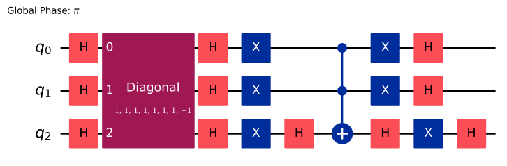
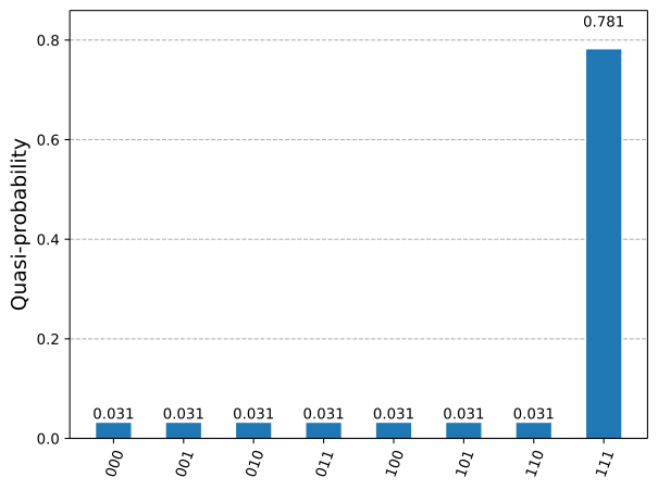
トランスパイラーが最適化を試みるための小さな回路を作成します。この例では、状態111をマークするオラクルを用いてGroverのアルゴリズムを実行する回路を作成します。次に、後で比較するために理想的な分布（完全な量子コンピューターで無限回実行した場合に期待される測定値）をシミュレーションします。

oracle = DiagonalGate([1] * 7 + [-1])
qc = QuantumCircuit(3)
qc.h([0, 1, 2])
qc = qc.compose(grover_operator(oracle))

qc.draw(output="mpl", style="iqp")

ideal_distribution = Statevector.from_instruction(qc).probabilities_dict()

plot_histogram(ideal_distribution)

トランスパイル

次に、QPU向けに回路をトランスパイルします。optimization_levelを0（最低）に設定した場合と3（最高）に設定した場合のトランスパイラーのパフォーマンスを比較します。最低の最適化レベルは、デバイス上で回路を実行するために必要な最低限の処理を行います。具体的には、回路のQubitをデバイスのQubitにマッピングし、すべての2Qubit演算を可能にするためにSWAPゲートを追加します。最高の最適化レベルはより高度で、全体的なゲート数を削減するためにさまざまな工夫を活用します。マルチQubitゲートはエラーレートが高く、Qubitは時間とともにデコヒーレンスするため、短い回路の方がより良い結果をもたらすはずです。

important

この例はIBM Quantum®ハードウェアを使用していますが、Qiskit互換の任意のQPUで試すことができます。結果は異なる場合があります。

次のセルでは、optimization_levelの両方の値についてqcをトランスパイルし、2Qubitゲートの数を出力し、トランスパイルされた回路をリストに追加します。トランスパイラーのアルゴリズムの一部はランダム化されているため、再現性のためにシードを設定します。

# Use Qiskit Runtime to run jobs on hardware
from qiskit_ibm_runtime import (
    QiskitRuntimeService,
    SamplerV2 as Sampler,
)

# Select the backend with the fewest number of jobs in the queue
service = QiskitRuntimeService()
backend = service.least_busy(
    operational=True, simulator=False, min_num_qubits=127
)
backend.name

'ibm_marrakesh'

# Need to add measurements to the circuit
qc.measure_all()

# Find the correct two-qubit gate
twoQ_gates = set(["ecr", "cz", "cx"])
for gate in backend.basis_gates:
    if gate in twoQ_gates:
        twoQ_gate = gate

circuits = []
for optimization_level in [0, 3]:
    pm = generate_preset_pass_manager(
        optimization_level, backend=backend, seed_transpiler=0
    )
    t_qc = pm.run(qc)
    print(
        f"Two-qubit gates (optimization_level={optimization_level}): ",
        t_qc.count_ops()[twoQ_gate],
    )
    circuits.append(t_qc)

Two-qubit gates (optimization_level=0):  21
Two-qubit gates (optimization_level=3):  12

CNOTはエラーレートが高いため、optimization_level=3でトランスパイルされた回路の方がはるかに優れたパフォーマンスを発揮するはずです。

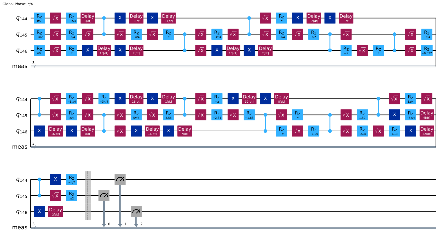
パフォーマンスをさらに向上させる別の方法として、ダイナミカルデカップリングがあります。これは、アイドル状態のQubitにゲートのシーケンスを適用することで、環境との望ましくない相互作用の一部を打ち消します。次のセルでは、optimization_level=3でトランスパイルされた回路にダイナミカルデカップリングを追加し、リストに追加します。

from qiskit_ibm_runtime.transpiler.passes.scheduling import (
    ASAPScheduleAnalysis,
    PadDynamicalDecoupling,
)

# Get gate durations so the transpiler knows how long each operation takes
durations = backend.target.durations()

# This is the sequence we'll apply to idling qubits
dd_sequence = [XGate(), XGate()]

# Run scheduling and dynamic decoupling passes on circuit
pm = PassManager(
    [
        ASAPScheduleAnalysis(durations),
        PadDynamicalDecoupling(durations, dd_sequence),
    ]
)
circ_dd = pm.run(circuits[1])

# Add this new circuit to our list
circuits.append(circ_dd)

circ_dd.draw(output="mpl", style="iqp", idle_wires=False)

回路を実行する

この時点で、異なる設定でトランスパイルされた回路のリストが揃っています。次に、SamplerプリミティブでこれらのCircuitを実行し、結果をresultに格納します。

sampler = Sampler(backend)
job = sampler.run(
    [(circuit) for circuit in circuits],  # sample all three circuits
    shots=8000,
)
result = job.result()

結果を表示する

最後に、デバイス実行の結果を理想的な分布と比較してプロットします。ゲート数が少ないためoptimization_level=3の結果が理想的な分布に近く、ダイナミカルデカップリングの効果によりoptimization_level=3 + ddがさらに近いことが確認できます。

binary_prob = [
    {
        k: v / res.data.meas.num_shots
        for k, v in res.data.meas.get_counts().items()
    }
    for res in result
]
plot_histogram(
    binary_prob + [ideal_distribution],
    bar_labels=False,
    legend=[
        "optimization_level=0",
        "optimization_level=3",
        "optimization_level=3 + dd",
        "ideal distribution",
    ],
)

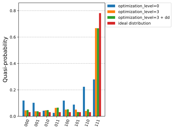
各結果セットと理想的な分布の間のHellinger忠実度を計算することで、これを確認できます（値が高いほど良く、1は完全な忠実度を表します）。

for prob in binary_prob:
    print(f"{hellinger_fidelity(prob, ideal_distribution):.3f}")

0.985
0.989
0.988

次のステップ

おすすめ

• 高度なトランスパイルのリソースを探索してみましょう。例えば：

  • カスタムトランスパイラーパスを作成する
  • カスタムバックエンドの作成とトランスパイル
  • トランスパイラープラグインのインストールと使用

• 利用可能なチュートリアルを参照してください。