クイックスタート

このガイドでは、qiskit-addon-obpパッケージの最小限の動作例を示します。演算子逆伝播(OBP)を使い、末尾のゲートをオブザーバブルに吸収させることで、量子回路の深さを減らします。

期待値$\langle O \rangle = \langle \psi | U^\dagger O U | \psi \rangle$は、回路$U$の末尾のゲートのブロックを取り除き、そのブロックでオブザーバブルを古典的に共役変換しても変わりません。OBPはこれを繰り返し適用し、回路の一部を古典的に評価することで、より浅い回路だけをハードウェアで実行できるようにします。代償として、吸収した各ゲートによってオブザーバブルがより多くのPauli項に拡大する可能性があるため、削減できる深さとオブザーバブルの増大を比較検討する必要があります。

このツールで現実的なワークフローを構築し、量子ハードウェアで実行する例については、IBM Quantum Platformのチュートリアル(OBPチュートリアル)をご覧ください。

OBPの入力を準備する

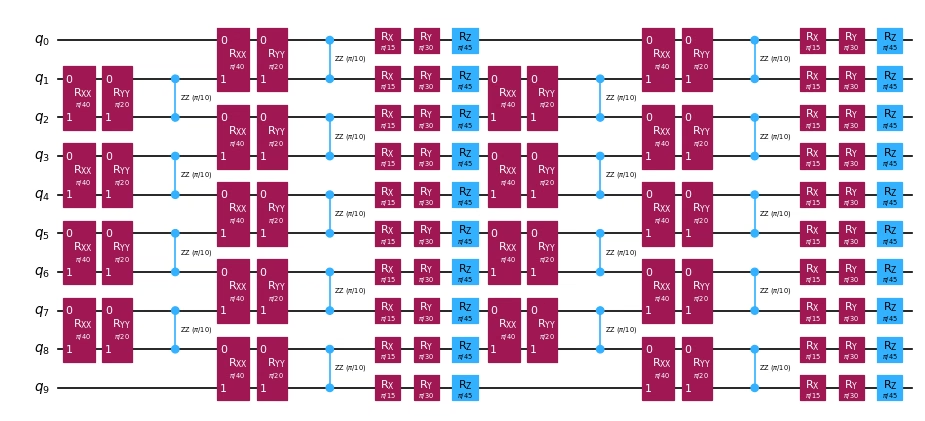
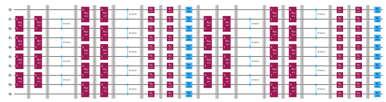
OBPは、回路スライスのリストとオブザーバブルを入力として受け取ります。回路の末尾からスライスを1つずつオブザーバブルに逆伝播し、オブザーバブルのPauli項が増える代わりに回路の深さを減らします。ここでは、10キュービットのHeisenbergモデルの時間発展回路を生成し、ゲートの種類ごとにスライスします。

以下では、元の回路を描画し、続いてスライスの境界をバリアで示して再結合した同じ回路を描画します。各スライスは、1回の逆伝播ステップでオブザーバブルに吸収できる単位です。

# Added by doQumentation — installs the packages this notebook needs if they are missing
import importlib.util

_needed = {"numpy": "numpy", "qiskit": "qiskit", "qiskit_addon_obp": "qiskit-addon-obp", "qiskit_addon_utils": "qiskit-addon-utils"}
_missing = [pip for module, pip in _needed.items()
            if importlib.util.find_spec(module) is None]
# One at a time, so a package that fails to install does not block the others
for _pip in _missing:
    %pip install -q {_pip}
if not _missing:
    print("\u2713 All required packages are installed")

import numpy as np
from qiskit.quantum_info import SparsePauliOp
from qiskit.synthesis import LieTrotter
from qiskit.transpiler import CouplingMap
from qiskit_addon_utils.problem_generators import (
    generate_time_evolution_circuit,
    generate_xyz_hamiltonian,
)
from qiskit_addon_utils.slicing import combine_slices, slice_by_gate_types

# Generate a circuit to reduce
coupling_map = CouplingMap.from_heavy_hex(3, bidirectional=False)
reduced_coupling_map = coupling_map.reduce(
    [0, 13, 1, 14, 10, 16, 5, 12, 8, 18]
)

hamiltonian = generate_xyz_hamiltonian(
    reduced_coupling_map,
    coupling_constants=(np.pi / 8, np.pi / 4, np.pi / 2),
    ext_magnetic_field=(np.pi / 3, np.pi / 6, np.pi / 9),
)

circuit = generate_time_evolution_circuit(
    hamiltonian,
    time=0.2,
    synthesis=LieTrotter(reps=2),
)

# Slice the circuit and define an observable
slices = slice_by_gate_types(circuit)
observable = SparsePauliOp("IIIIIIIIIZ")

print(f"Original circuit depth: {circuit.depth()}")
print(f"Number of slices: {len(slices)}")
print(f"Observable terms: {len(observable)}")

Original circuit depth: 18
Number of slices: 18
Observable terms: 1

# Recombine the slices with barriers to make the slice boundaries visible
sliced_circuit = combine_slices(slices, include_barriers=True)

print("Original circuit:")
display(circuit.draw("mpl", scale=0.6, fold=-1))
print("Sliced circuit (recombined with barriers for visualization)")
sliced_circuit.draw("mpl", scale=0.6, fold=-1)

Original circuit:

Sliced circuit (recombined with barriers for visualization)

OBPで回路の深さを減らす

backpropagateを呼び出して、スライスをオブザーバブルに吸収させます。この関数は、拡張されたオブザーバブル、逆伝播されなかった回路スライス、およびこの手順に関するメタデータを返します。

制限しないと、オブザーバブルは$2^n$個のPauli項に向かって増大しかねません。operator_budgetはこの増大に上限を設けます。ここでは、キュービット単位で可換なグループを最大8個まで許可します。これは、QPU上でオブザーバブルを評価するために必要なショット数をおおよそ決めます。次のスライスを吸収すると予算を超える場合、逆伝播はその時点で停止します。以下ではまさにそれが起こっており、オブザーバブルが8個の可換グループをすべて使い切った時点で、18個のスライスのうち7個だけが吸収されて手順が止まります。

回路のさらに深くまで進めるには、backpropagateのキーワード引数truncation_error_budgetを使い、オブザーバブルが増大する際に係数の小さいPauli項を切り捨てることができます。これにより、切り捨てるPauli項の大きさに比例する誤差と引き換えに、オブザーバブルの増大を抑えられます。2つの予算は補完的で、併用できます。operator_budgetはオブザーバブルのサイズを制御し、truncation_error_budgetは項を捨てることで生じる誤差を制御します。

from qiskit_addon_obp import backpropagate
from qiskit_addon_obp.utils.simplify import OperatorBudget

max_qwc_groups = 8
bp_obs, remaining_slices, metadata = backpropagate(
    observable,
    slices,
    operator_budget=OperatorBudget(max_qwc_groups=max_qwc_groups),
)

reduced_circuit = combine_slices(remaining_slices)
num_groups = len(bp_obs.group_commuting(qubit_wise=True))

print(
    f"Backpropagated {metadata.num_backpropagated_slices} of {len(slices)} slices."
)
print(
    f"Reduced circuit depth: {reduced_circuit.depth()} (was {circuit.depth()})"
)
print(f"Observable grew from {len(observable)} to {len(bp_obs)} Pauli terms.")
print(
    f"Filled {num_groups} of {max_qwc_groups} commuting groups, exhausting the budget."
)

Backpropagated 7 of 18 slices.
Reduced circuit depth: 11 (was 18)
Observable grew from 1 to 18 Pauli terms.
Filled 8 of 8 commuting groups, exhausting the budget.

reduced_circuit.draw("mpl", scale=0.6, fold=-1)