原子核ハミルトニアンのプール型サンプルベース量子対角化
使用量の目安: Nighthawk r2プロセッサーで32秒(注: これはあくまで目安です。実際の実行時間は異なる場合があります。)
学習目標
-
軌道の結合基底で表形式にまとめられた原子核殻模型ハミルトニアンが、1つの量子ビットが1つの単一粒子状態に対応するスキームの量子ビットハミルトニアンになる仕組みを学びます。
-
角度が2次摂動論から得られる、固定された非変分の励起アンザッツを構築します。そのため、古典的な最適化ループは不要です。
-
量子ビット励起とフェルミオン励起を比較し、その選択がアンサンブルの2量子ビット深さにどう影響するかを測定します。
-
保存量が電子数とスピンではなく、核子数、、パリティである場合に、
qiskit-addon-sqdを使って自己無撞着な配置回復を実行します。 -
正確に検証できる24量子ビットの問題から、このチュートリアルの厳密対角化の能力を超える、約200万の基底状態を持つ40量子ビットの問題まで、1つのワークフローを適用します。
前提知識
始める前に、次のトピックを確認してください。
-
化学ハミルトニアンのサンプルベース量子対角化。このチュートリアルの電子構造版にあたります。
-
第二量子化とJordan-Wigner写像。
背景
原子核殻模型は、原子核を、不活性なコアの上にある少数の単一粒子軌道の中を動く数個の価核子として扱い、測定されたスペクトルに合わせて調整した経験的な二体力を通じて相互作用させます。低エネルギー原子核構造で広く使われています。その計算コストは組合せ的に増大します。基底は、価陽子と価中性子を利用可能な状態に分配するあらゆる方法からなり、この増大が厳密対角化で扱えるモデル空間を制限します。
プール型サンプルベース量子対角化(プールSQD)[1]は、この問題を2つに分割します。量子回路は、どの基底状態が重要かを提案するためだけに使われます。計算基底で測定し、測定された各ビット列が1つのスレーター行列式を表します。その後、ハミルトニアンは、それらの行列式が張る空間で古典的に構築され、対角化されます。古典的なステップは部分空間内での厳密対角化であるため、真の基底状態エネルギーに対する変分上界を返し、この上界は行列式を追加するにつれて下がることしかありません。
この役割分担により、この手法はノイズ耐性を持ちますが、重要な制限があります。ノイズが変えるのは、回路がどの行列式を提案するかだけです。ノイズは古典的なハミルトニアンには入らないため、与えられた部分空間の固有値を動かすことはできません。保存量に違反したショットは破棄または修復され、生き残ったショットは、どのように生成されたかにかかわらず正当な基底ベクトルです。したがって、ノイズが損なうのは部分空間の質であって正しさではなく、報告される値はいずれの場合も上界です。
原子核構造は、サンプルをフィルタリングするための厳密な量子数をいくつか提供します。物理的な行列式は、正しい数の価陽子と正しい数の価中性子、正しい全角運動量射影、そして正しいパリティを持たなければなりません。それぞれはビット列に対する整数テストで確認できます。棄却されるサンプルの割合は、制約とモデル空間によって異なります。
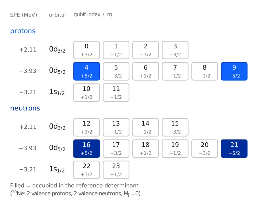
すべての量子ビットは1つのスキーム単一粒子状態であり、は占有を意味します。レジスターは固定された順序を使います。まず陽子、次に中性子の順で、同じ種類の中では軌道はファイルの順、1つの軌道の中ではの降順です。したがって、ビット列の2つの半分は、それぞれ陽子配置と中性子配置になります。これは、プールSQDの後処理ツールが想定する2分割です。
ワークフロー
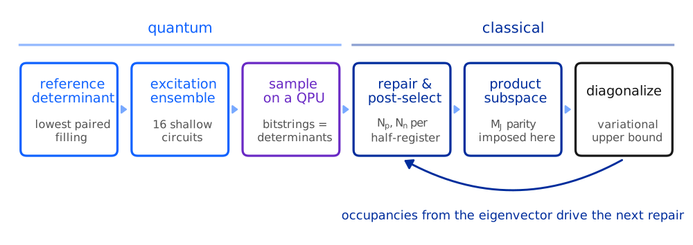
図の2つのステージが、原子核の対称性を扱います。
修復と事後選択は、ハードウェアノイズの影響を受けたサンプルを扱います。レジスターの各半分の核子数はハミング重みなので、qiskit-addon-sqdが直接扱えます。recover_configurationsは、壊れたビット列を、ショットを捨てるのではなく、平均軌道占有数の現在の推定値と最も整合しないビットを反転させることで修復します。
積部分空間ではを導入します。は2つの半分を結合するため、どちらか一方の性質ではなく、ショット全体のフィルタリングに使ってはいけません。陽子の半分と中性子の半分がそれぞれ有効なビット列は、全体のが間違っていても、2つの有効な半分の配置として寄与します。したがって部分空間は、サンプルされた陽子配置とサンプルされた中性子配置のあらゆる積で張られ、目標のとパリティのセクターに入る積だけを残します。これがプールSQDの部分空間の構成であり、数千のビット列が、サンプル数よりはるかに大きな部分空間を張れることを意味します。
2つの支配方程式
殻模型ハミルトニアンは、1体項と2体相互作用の和です。
ここではスキームの状態を表し、陽子では、中性子ではです。USDA [2]やGXPF1 [3]といった経験的相互作用は、スキームではなく結合基底で、軌道の規格化・反対称化された2体状態間の行列要素として表にまとめられています。スキームの要素を復元するには、Clebsch-Gordan再結合を行います。
の因子は、表にまとめられた状態の規格化の規約を打ち消します。このチュートリアルの他のすべては、この2つの方程式の上に成り立っています。
3つの実行
| 原子核 | 殻 | 量子ビット | 対称性で許される基底 | 厳密に検証可能か | |
|---|---|---|---|---|---|
| 小規模 | (2p + 2n) | 24 | 640 | はい | |
| 大規模 | (2p + 2n) | 40 | 4,000 | はい | |
| 大規模 | (4p + 4n) | 40 | 1,963,461 | いいえ |
小規模な実行はウォークスルーです。2つの大規模な実行はどちらも40量子ビットのレジスターを使います。1つ目はノートPCでも厳密に対角化できる規模なので、ハードウェアの結果を厳密な参照値と比較できます。2つ目は、このチュートリアルの厳密対角化の能力を超えています。
**ここでのすべての実行はQPU上で行われます。**これは手法の要件ではなく、このチュートリアルのための選択です。3つの実行はバックエンドとゲート予算を共有するため、問題サイズごとの性能を比較できます。
要件
始める前に、次のパッケージをインストールしてください。
-
Qiskit SDK v2.0以降(
pip install qiskit) -
qiskit-ibm-runtimev0.40 or later (pip install qiskit-ibm-runtime) -
SQDアドオン v0.12以降(
pip install qiskit-addon-sqd) -
NumPy、SciPy、Matplotlib(
pip install numpy scipy matplotlib)
また、認証情報がローカルに保存されたIBM Quantum®アカウントと、40量子ビット以上のQPUへのアクセスが必要です。
シミュレーターのパッケージは不要で、データファイルをダウンロードする必要もありません。このチュートリアルで使う2つの相互作用ファイルは、次のセットアップセルに埋め込まれており、実行すると一時ディレクトリに書き込まれます。
セットアップ
このセクションでは、ワークフローが使う順に、ツールをインポートし、殻模型のヘルパーを定義します。それぞれの背後にある物理は付録で導出されています。コメントでは、ワークフローにおける各関数の役割を説明しています。
まず2つの相互作用ファイルを展開します。どちらも公開されているパラメーターセットで、ノートブックが自己完結するようここに埋め込まれています。usda.sntはUSDA 殻ハミルトニアン [2]、gxpf1.sntはGXPF1 殻ハミルトニアン [3]です。
# Added by doQumentation — installs the packages this notebook needs if they are missing
import importlib.util

_needed = {"matplotlib": "matplotlib", "numpy": "numpy", "qiskit": "qiskit", "qiskit_addon_sqd": "qiskit-addon-sqd", "qiskit_ibm_runtime": "qiskit-ibm-runtime", "scipy": "scipy"}
_missing = [pip for module, pip in _needed.items()
            if importlib.util.find_spec(module) is None]
# One at a time, so a package that fails to install does not block the others
for _pip in _missing:
    %pip install -q {_pip}
if not _missing:
    print("\u2713 All required packages are installed")
from __future__ import annotations

import base64
import gzip
import itertools
import tempfile
from dataclasses import dataclass
from functools import lru_cache
from math import factorial, sqrt
from pathlib import Path

import matplotlib.pyplot as plt
import numpy as np

from qiskit import QuantumCircuit
from qiskit.circuit.library import PauliEvolutionGate
from qiskit.quantum_info import Operator, SparsePauliOp
from qiskit.transpiler.preset_passmanagers import generate_preset_pass_manager
from qiskit_addon_sqd.configuration_recovery import recover_configurations
from qiskit_addon_sqd.counts import bit_array_to_arrays
from qiskit_addon_sqd.subsampling import postselect_by_hamming_right_and_left
from qiskit_ibm_runtime import QiskitRuntimeService, SamplerV2

from scipy.linalg import eigh

_USDA_SNT_GZ = (
    "H4sIAI5wqWoC/4WY224bRwyG7/UU9F0CONsZco5AUyBuC/QmQNG06KWhWGql1LYMy+kJefiOTrucGXJrQAgsf5nl8ecOr+CX"
    "D9+9g/0K9pv1/T389rx7gPLrsH+Cz/vVctg+vgAsrgB+HeDdAD9t7zYv6+dr+DDA+z8223/X17B8XMFN+ev9+m+4ed799XjA"
    "f9z8sy/4+s8BvoWYrsEERwbhFRqTXi+uCvOwW63vYf+0vFvDAgDo/AFIh8/hK7DH30354Omvb8o3V8c/vIUnMKtboK/wiGKF"
    "+gnFEfVn9PQUe8bthNIRtftbsGfUtQbAGXUFfawM8K0BF9SP6MWA0BpwQcMRvRhwBSX86+fl3ct2d4jq4+eHa3hYv2x2q7fX"
    "AJuPy+fb3cP69+Uh4luAT8djv95++eGV/fj6y6dvFudnmcX4lGOoBmttNOVncTL2FLs3NGT0l++ndJTv0cR8/t6NUanP8WMI"
    "6nPC6C8/5wp+vnn//QLOP9ank3k2wRszkDn/Zwv15xiv41l2SDmjhuEFM4PJ0QkYcgzM4A1Jp1GDkcvtaWMAR9tosAa9huHk"
    "AtoUBYwaF8hGarAxOywgxnoeN+Se2smF4H3QMPZQ653XMJpOi6GyrcLcZJtzLgoYcdsOyXKibV1Aom0fikJO0VLUMDeW3kAl"
    "qQLWpd66qGE02eZ9lXqSPD3UWyl5DeOeGnINJnmaUggCVrtgh2DJNm3fVy8WF3LSMFa9hYga5iYX0IQsYK2nmTpJkoq81Acy"
    "jLTTnPEaxqo3JGcbvZMeGnJVbw6mf2cUqcIsO80nFdOFq8JoSlY+Zb7FfNNZlnw2PqOE8SL3PtlSJhJGXGqsDRjbh4bmocWy"
    "oiIxSxjv09JYgaxlGLZxA9EFFOImuIBt3EB04TK3Z5S8wizrrFCJQ4Xpgl9hzDYbu0LCNm6HzkJHweUkYazITalyF7NjGAnh"
    "FZJFQniFZFHnqWgbdZ6qtoX50VZhvEJ81TJe7AUcQozH8yQMJ8ymUS07jLin6LXT3FRIhmwSTmtbJpEjr2AsvM7E1ra+ZaiM"
    "NoxewZinBlPQTmPJyikn7TQ2630SbWuz4CLlwzuGhCHPqbUmRZQwpkiBDn1vsoQ55oKjbEvNNVgbXls0WvA0NKnPpku91Fkx"
    "pahhXPDJtxVCQkBcMtJD27I8VJGAhWYYlVuZzc5e+jSIZWnLa57nOQ1iWZY+jSE3GP5/QIKi5E1Agqi9BbMZiUjEWNwChqKq"
    "KTZY11ku5ca2Pqc4YKk1o2DstBjJC1htW2nAgEZ4aDdPvQmmmLeY4tWFt9Y3VAdlpW+oDcpa3zpM1jdUB2XV9agOyqrrcWZQ"
    "sq7vMMffBseux5l5yjoLZ+Yp6yzU5mmt5DgzT5mSozZPoVIknJmnTJFQHZRV12OrlvpFQFbycoGKOWiYfl9QlXySGtSUvL9W"
    "VJi/YG4grC4CmuCX6CZrKUsY64UyJolCQoZJqWeKhDOCzxQJNcGXbZMEX7EtzF+gvCI1npxjmKaW5Q06ewVjOY0u2+Y0kt5D"
    "JhlETS2P+5CqyIMYkCI1NK50SO3TarSR2qfVaKOZPmXjg2beVJmS01zqp/CSmvoqvNSOD/kaS+qUoSGaTM2yz83fdjtMvsZy"
    "xOv7N44Fff/GT5q5tXWYfB3jWND3b9yumUvK5SQnvK6w/VuHyfu3DpP3bx0m7984FvT9W4fJ+zceWq/v3zpM3r9xLOj7tw6T"
    "928X053QgGz/1mHy/u3yZ8lTtn/jWND3b74NiDx2vRbeep56Lbz1oPRaeOv9G0dmxofXPK33bx0m798C1B9RuP4DPJ0WcLAa"
    "AAA="
)

_GXPF1_SNT_GZ = (
    "H4sIAI5wqWoC/4WcQY8dtw3H7/kU41sCeF8lUqKkQw9NgbaXoEHQQ26BkdiIEWdt2E6L9tNXb9+ORIn8PwdZILB/S3I4IsW/"
    "ZiYvjr//+P3f4nG8ef/x+PDm4dOvr9+9++rF8d3l+Mf7x99fvTz+dTn++fnTH7/1//z28pfL8e3H9/95fHm8evzl+lffvf3f"
    "H59e/fb26L9zHN//+t9Pl+OH1/++HH89JL88gkQO8esfvjm+phDomyvW//39/S+v3x2fPrz6+fVX/dfS889B4fpz/aN43P7p"
    "f3Bw/ynH8fD0Zy+uf/fn48MR3vxU/kRXlp7Z+PzDiqUnNn74iW8sb3azYvm0m29s2uxGxabTbryx2cZ7nGzu7KOKV2y8g5Un"
    "dsZbbLyDLafd53irjXew9bR7jffF8fbx8+uPr37+/Pb941dPv3P93ZH4W/If6kUohXCm+Jbmh3yR0jicybwl9CFeuFILy908"
    "HtIlcrlZyCNJ2q6MdGi7ZVy4tlvHJS52Y71FnHp8D+HCIYTlQuYFhdsv0yVxzZB6vsxwaZwJUumkIjWB1POdDhcqlR2KVo85"
    "SoDU8NgdNodiZevqMUqB1LCVWsO2ZMQlyYs+bXEFk4m5bMJJlVgSpGjaouhQvFKxUIbUjIvI85hWW4FNvubyDnMxMkFKRc8V"
    "Uml65OhQW1x9fe3XOAtsZPXJ36TIX18SaoQUnysnZsHUXPfcKqTyaSu36FHbWg0tN0jxWIXEAVLzbqcqkMpj3T8lwlBp9RhD"
    "qpAaHpnzni9nRXPh6lDbysmJBVLzDtU71KztnDxqW1+JhDaKnTtUa4DUzH00Hp0VXQMHSM3c16irlpf7GEcN1dogpfpEDpAa"
    "WRUOBKl0UqkIQ2qs+5IYU6OvthbFodIaF6/9i51VeF0TLZSN2lfh9T729utQOqtXKi/dl/21mihhW+M+BpIKqblypDWHSntc"
    "mSA1O3nMe+6dHp0DEaRmXCU0h9p7dOYCqVm1MehOnvy7nWphSKnuu+Q++X2Ca4uQGrYkxp3yMkFLL0ygavPovmR64dhFY5QM"
    "KVK1XRxqX4UydlHCXU44hY1ydndKuUBK11BzqH1NNOKNMvt27PMXVUWBemSqCVIjrr4nYFtzTSQJkJp3O7se09p9YygCKVL7"
    "UN4opx5DNnE5q5AlerZ2jyExpEYmggTtMYFrzC1Bak58jetGeSvHenSip9ROik0m5lqdsxzjrCYhTM1uImOHYZzVPvnWjXIm"
    "0RoaKyqhjjlqiEE3uWoYHqopbT/KY0pDD+Xtx9d8lvI0n6U8zWcpT/NpQqDms5Sn+TRVoOazlKf5LOVpPk1VqPl05AI1n6U8"
    "zaepAjWfpTzNp6kKNZ/OQoGaz1Ke5rOUp/k0VaHm03mvUPOd1+esL6X5LOVpPkt5ms9SnubTVIGaz1Ke5rOUp/ks5Wk+TVWo"
    "+SzlaT69mgVqPk0VqPks5Wk+S3maT1MVaj5dPwVqPkt5mk9TFWo+S3ma77x/8z56ms9SnuazlKf5LOVpPkt5ms9SnubTVIWa"
    "z1Ke5jupfRWumk9TBWo+S3maz1Ke5rOUp/k0VaHms5Sn+XTnLVDzWcrTfJqqUPNZytN85/1z7rbSfJbyNN/5t06fUJrPUp7m"
    "OykvE7T0wgqqdmo+Mb3Q03yCO6bSfII7ptJ8gruc0nxi+pen+eROL5yaT3CXU5pPx1Sh5hNcj0rzCajHVfMJqMdV88mdesyu"
    "xwo1n+B6VJpPcD0qzSe4HpXmE1yPSvMJrkelwERVR4Waz1Ke5hNTQ3THoxO90nzFZMLTfAVnVWm+grOqNF/BWVWaTxMVar6C"
    "r1FpvgK6yar56vbja76onormu8/5ViqOrNblZH6l0NPAlRq9sKaIbaFnhis15tUuH/E1oieLK1XOTIgsz3ROap9XpQ/SJWqK"
    "bCYcKm6K4tp9iUqqzbd1j4qO+g2tpTV6sll1qLipk6fnw32/isDWPSruPborwz7x9eakKbbry6Gi7RN9nrhuHr4tPXXsVLT9"
    "vvTdKlUQ18i9Q0Wn+2ZOlYpva0yiDhXthNz69p4S+7ZG7h0q2jma+/BIIfm2RnU4VLQ9R6hG4iWryVurhorOlNbzEJr4tubk"
    "bim6e25iqbFbJY4MKfREfaXGNXKK2aF2BSapD6Oy5162yd1S5Og0iq3k5tua1WEpsus+ZO4ZS76tqU4sRc7+mAtJyL6teR8t"
    "RVbDUO9yXM2a2O6jQ5GjdCi3HKpva04dluK7J1uWGtFLjhFS6J2HlZpKhzOm0JsRK5XnmjD7Izv5av0eBd7zVb5IsVU6ffTN"
    "oQXf1peoeveNjZWaNURFZ0L8fTsX1s9hwO4eeHkOA3Z3Zct6ZOccgPAM0O91hR4ZPEcWMAPkdBWQvsdZj72xZuTRs2U95qFY"
    "a8FZHVQpy/Mhd55YbGmPew2VGB2PRvOVsNlib0orYbO1U8fi0cbF6uQhw7jUycMybYs/dSiKwGxyLB5tXEmdM5WM4lKnGLFm"
    "FFeaPTruK8ehlEcbV55n2yIwrnlOXorAuPKsxyIwrjz7l3greptzSgve+tqo2lLbcu9MQ4oiPDMpjzaueR8rUUZxqaql/T46"
    "k5WiCM9fyuNpy5uZpM9WkvfaxpS1Ndd96JKV2LflUdrW1idaKOT0HNMnTCdnT/OZvcOZv5RHG5fqAJFhXLO2WykwrtlzJkV4"
    "llMebVxp7kOUMopr7h1dSmcUl9LuxesT2z6kPOq4ttkkk7sj1/1JWWWnHvfdfVKE50LlUV+jObPqs2hO+zViytpSJ+CFSyu+"
    "LY+yttRM3gf3HH1bHmVtzR5NXZQXcI0epW1tdyh2d86a2O52F9vR6V8FUgTm1dWjjWuepZUgMK45k2cKMC6PIjD7rh6j+gpi"
    "0Y904b675/n2h3u6QteTedkoc7qy2LIeaUxpkXNAHgeV53khozOYxZb1qDpTrvAa+TxBClECvEbPlvWY5o4cA7zGNDSfFIbX"
    "6NmyHmd1SEnwGgfVJ6YKr9GzZT3KebdDZIYe5bzGQLFAj54t7XHXfDkmJ6v789r17e7iTEMrxXhmUh5tXHNmainCuObMVBOO"
    "y6MYzEyrx9MW2VMf4cC9NWlbzpmVoqytucPkIO12SsZ4/lKUtTX7V6LGsfi2phadlLa1nX89naUHc437uYnQni/nlEzWN/S8"
    "s7TVo41LvUsW9+pwqFBl79HsPYkVr/sK9GjjYnVWSzBfqjoowXx5FN+ZC6dHG5d6WybjfM15ouYE8+VRDObC1aOOa3v+WEJq"
    "Tlzb2VCRELOtbYEU47NH5dHGpd5nagzj0s+HAozLoxjMq6tHnfutHmNjblz23G/1qChra3rMOT6f3jGefRVlbamZKfR1COKa"
    "PWdS1tZcXy3mnMm3pd4IGpS1Nd9Uai0Wir6t+fxxUtrWPvu27M1MG8XJ1KMz+yqK8Vmt8mjjmn1CKmcUF88zhVIzimtOtZNi"
    "fO6rPGpbW9XGLrg50G5rfwNhUueu7swmEtI55yQ0m/RpqI3JPd15ujVtWY9TSbcxpSU8dSShAj16tk4b3r6dmUlI2/L27Ulp"
    "W7vKLFK3uByK4nI2VP19SFEJ7EOrRxvXyESr413YhPchLsssV/0dRlEJ70PKo7a1n/vWa1rLbsu8mTooa0up8tpyEd+Wep42"
    "KG1rf6su5ebkvpqztLzl3qltRSVc28ojmTM+9F2TwNm3Qgp9/eSeKnaNXFtwqH3nk1KaJE05M6ZDOdNjv9NJIvm2Zr+3lFeP"
    "EvqGnH1bM/eWMtNQvFCRHnzUlJlzXMqZYFKqHHLxbdFUFIbiu+8XWmo+50vL6R06l1u/PBO/asN8B5zAmdXTDtP7r8h+jeWL"
    "lFOPocYumti39SWq3v0iTvxdtDw9hhmUq9N6PbaqvzJyqyNeMi0nIm51LLbojgIrOUKP+l2yBj16tghrqxib1gqg0pLknfIq"
    "bdoirJqkMMNrnDNATPgaPVuE9VBv0J7HbU107V42W44eUhSjPrF4JKyHUokZxqXeTV+exAI9pCjGp/zKIwE9dO2+XSTX1vbc"
    "b6pJUYT1UOCWWw2+rdmZJkVYD1Ef0Uoi39acySdFWA9RztLVjm9LPQ0cFAENc3unJjrVsWuY0mK297EYxbrbcs7vlUfCGib3"
    "bQ/GNWffMijCGkZRDHr0w+KRsIbpnem6dnZbe9VOitTsW7e3I+e7Pgnv7tfHQxvl7O7KlvU4zu95fouUUNV21RSGFk2oHhdb"
    "ZGbf+b4cXf8nRlnb8maASVlbc+UkSnSb0hKox4eFIjNHz7c/aHydkvC6T9Lydo3Je+u8ZSdf+xsu06O2ta2vPr70W1l2W9v6"
    "UhSbPoG+kwYnSDVnTKGvqYvfv3JuDVLom2vvpOZpvh9fizHuX71jVp79vqDcG8rrJolLnecTxe8TgMLfBTDoJteOGUVntYJr"
    "5PHOVsKnUaEuJw8oE9MWA5V5e2tA9wmQrw5xQB6RrernS33VkEB1PCmKW5f7P6zudeW7TwAA"
)

DATA = Path(tempfile.mkdtemp(prefix="nuclear_sqd_"))
for name, blob in (("usda.snt", _USDA_SNT_GZ), ("gxpf1.snt", _GXPF1_SNT_GZ)):
    (DATA / name).write_bytes(gzip.decompress(base64.b64decode(blob)))

    if not (DATA / name).is_file():
        raise RuntimeError(f"{name} did not unpack to {DATA}")
モデル空間と量子ビットレジスター
.sntファイルには、モデル空間、単一粒子エネルギー、結合の2体行列要素が含まれます。ここで使う質量依存の相互作用では、2体ヘッダーの3番目と4番目のフィールドが、相互作用がフィットされた基準質量と、その質量依存の指数を指定します。どちらのファイルも指数はで、はUSDAでは18、GXPF1では42です。したがって、表にまとめられた行列要素は、計算対象の原子核に合わせてでスケールし直す必要があります [2]、[3]。単一粒子エネルギーはスケールし直しません。この手順を省くと、相関エネルギーが数パーセント変わります。
以下のエネルギーは、不活性なコアから測った価エネルギーであり、実験的な分離エネルギーではありません。
@dataclass(frozen=True)
class Orbital:
    idx: int
    n: int
    ell: int
    j2: int
    tz: int  # j2 = 2j; tz = -1 proton, +1 neutron

@dataclass(frozen=True)
class SPState:
    """One m-scheme single-particle state, i.e. one qubit."""

    orb: int
    j2: int
    mj2: int
    tz: int
    ell: int
    spe: float  # mj2 = 2 * m_j

@dataclass
class ModelSpace:
    orbitals: list
    spes: dict
    tbmes: dict
    core_z: int
    core_n: int
    mass_number: int
    a_ref: int
    mass_exponent: float
    mass_factor: float

def read_snt(path, n_protons, n_neutrons):
    """Parse a .snt interaction file, applying its mass dependence for this nucleus.

    The two-body header line is ``n_tbme  method  A_ref  exponent``.  When ``method`` is 1 the
    tabulated matrix elements are rescaled by ``(A / A_ref) ** exponent``, where A is the mass
    number of the whole nucleus -- the core plus the valence nucleons.  A is derived from the
    file's own core numbers rather than passed in, so it cannot silently disagree with the
    valence counts the rest of the workflow uses.  Single-particle energies are not rescaled.
    """
    rows = [
        ln.split("!")[0].split() for ln in Path(path).read_text().splitlines()
    ]
    rows = iter([r for r in rows if r])

    n_p_orb, n_n_orb, core_z, core_n = (int(x) for x in next(rows)[:4])
    orbitals = [
        Orbital(*(int(x) for x in next(rows)[:5]))
        for _ in range(n_p_orb + n_n_orb)
    ]

    spes = {}
    for _ in range(int(next(rows)[0])):  # "i  i  <i|H(1b)|i>"
        field = next(rows)
        spes[int(field[0])] = float(field[2])

    n_tbme, method, a_ref, exponent = next(rows)[:4]
    n_tbme, method, a_ref, exponent = (
        int(n_tbme),
        int(method),
        int(a_ref),
        float(exponent),
    )
    mass_number = core_z + core_n + n_protons + n_neutrons
    factor = (mass_number / a_ref) ** exponent if method == 1 else 1.0

    tbmes = {}
    for _ in range(n_tbme):  # "a  b  c  d  J  value"
        field = next(rows)
        tbmes[tuple(int(x) for x in field[:5])] = float(field[5]) * factor

    return ModelSpace(
        orbitals,
        spes,
        tbmes,
        core_z,
        core_n,
        mass_number,
        a_ref,
        exponent,
        factor,
    )

def m_scheme_states(ms):
    """The qubit register: protons then neutrons, orbitals in file order, m_j descending."""
    return [
        SPState(o.idx, o.j2, m2, o.tz, o.ell, ms.spes[o.idx])
        for tz in (-1, +1)
        for o in ms.orbitals
        if o.tz == tz
        for m2 in range(o.j2, -o.j2 - 1, -2)
    ]
Clebsch-Gordan再結合
式(2)には、半整数の角運動量に対するClebsch-Gordan係数が必要です。すべての引数は物理的な値の2倍で渡されるため、は5として入力され、演算は厳密なままです。
Interaction.v_msは、相互作用の行列要素の検索を処理します。.sntファイルは各行列要素を1度だけ格納するため、検索では、いずれかの側で反対称化された対交換の位相が必要になる場合があり、ブラとケットはどちらの順序で格納されていることもあります。
@lru_cache(maxsize=None)
def clebsch_gordan(j1_2, j2_2, J_2, m1_2, m2_2, M_2):
    """<j1 m1 j2 m2 | J M>.  Every argument is twice its physical value."""
    if m1_2 + m2_2 != M_2 or not abs(j1_2 - j2_2) <= J_2 <= j1_2 + j2_2:
        return 0.0
    if abs(m1_2) > j1_2 or abs(m2_2) > j2_2 or abs(M_2) > J_2:
        return 0.0
    if (j1_2 + j2_2 - J_2) % 2 or (j1_2 - m1_2) % 2 or (j2_2 - m2_2) % 2:
        return 0.0

    f, half = factorial, lambda x: x // 2
    prefactor = sqrt(
        (J_2 + 1)
        * f(half(j1_2 + j2_2 - J_2))
        * f(half(j1_2 - j2_2 + J_2))
        * f(half(-j1_2 + j2_2 + J_2))
        / f(half(j1_2 + j2_2 + J_2) + 1)
        * f(half(J_2 + M_2))
        * f(half(J_2 - M_2))
        * f(half(j1_2 - m1_2))
        * f(half(j1_2 + m1_2))
        * f(half(j2_2 - m2_2))
        * f(half(j2_2 + m2_2))
    )
    total = 0.0
    for k in range(half(j1_2 + j2_2 - J_2) + 1):
        d = [
            half(j1_2 + j2_2 - J_2) - k,
            half(j1_2 - m1_2) - k,
            half(j2_2 + m2_2) - k,
            half(J_2 - j2_2 + m1_2) + k,
            half(J_2 - j1_2 - m2_2) + k,
        ]
        if all(x >= 0 for x in d):
            total += (-1) ** k / (
                f(k) * f(d[0]) * f(d[1]) * f(d[2]) * f(d[3]) * f(d[4])
            )
    return prefactor * total

class Interaction:
    """Antisymmetrized m-scheme two-body matrix elements <pq||rs>, per Eq. (2)."""

    def __init__(self, model_space, sp):
        self.ms, self.sp, self._cache = model_space, sp, {}

    def _tbme(self, oa, ob, oc, od, J, j_ab_2, j_cd_2):
        """<oa ob; J|V|oc od; J>, allowing for how the file happens to order each pair."""
        table = self.ms.tbmes
        # |ba; J> = -(-1)^(j_a + j_b - J) |ab; J> for a normalized antisymmetrized pair;
        # dropping the leading minus makes v_ms symmetric instead of antisymmetric, and
        # the Hamiltonian then fails the rotational-invariance check in Step 1.
        phase_ab = -1.0 if (j_ab_2 // 2 - J) % 2 == 0 else 1.0
        phase_cd = -1.0 if (j_cd_2 // 2 - J) % 2 == 0 else 1.0
        for keys, phase in (
            (((oa, ob, oc, od), (oc, od, oa, ob)), 1.0),
            (((ob, oa, oc, od), (oc, od, ob, oa)), phase_ab),
            (((oa, ob, od, oc), (od, oc, oa, ob)), phase_cd),
            (((ob, oa, od, oc), (od, oc, ob, oa)), phase_ab * phase_cd),
        ):
            for key in keys:
                value = table.get(key + (J,))
                if value is not None:
                    return value * phase
        return 0.0

    def v_ms(self, p, q, r, s):
        """<pq||rs>, zero unless M_J and charge are conserved."""
        cached = self._cache.get((p, q, r, s))
        if cached is not None:
            return cached

        P, Q, R, S = (self.sp[i] for i in (p, q, r, s))
        value = 0.0
        if P.mj2 + Q.mj2 == R.mj2 + S.mj2 and P.tz + Q.tz == R.tz + S.tz:
            M = P.mj2 + Q.mj2
            # sqrt(1 + delta): undo the normalization of the tabulated pair states
            c12 = sqrt(2.0) if (P.tz == Q.tz and P.orb == Q.orb) else 1.0
            c34 = sqrt(2.0) if (R.tz == S.tz and R.orb == S.orb) else 1.0
            for J2 in range(
                max(abs(P.j2 - Q.j2), abs(R.j2 - S.j2)),
                min(P.j2 + Q.j2, R.j2 + S.j2) + 1,
                2,
            ):
                cg_bra = clebsch_gordan(P.j2, Q.j2, J2, P.mj2, Q.mj2, M)
                cg_ket = clebsch_gordan(R.j2, S.j2, J2, R.mj2, S.mj2, M)
                if abs(cg_bra) < 1e-12 or abs(cg_ket) < 1e-12:
                    continue
                value += (
                    c12
                    * c34
                    * cg_bra
                    * cg_ket
                    * self._tbme(
                        P.orb,
                        Q.orb,
                        R.orb,
                        S.orb,
                        J2 // 2,
                        P.j2 + Q.j2,
                        R.j2 + S.j2,
                    )
                )

        self._cache[(p, q, r, s)] = value
        return value
行列要素と対称性テスト
行列式は、占有された量子ビットのインデックスをソートしたタプルです。占有状態が2つより多く異なる2つの行列式の行列要素は0になります。そうでなければ、Slater-Condon則により、相互作用についての短い和が得られ、固定されたレジスターの順序で演算子の間にいくつの占有状態があるかを数えるフェルミオン符号が掛けられます。
symmetry_allowedは、4つの厳密な量子数すべてが帰着する整数テストです。サンプルのフィルタリングと、検証可能な小さな実行のための厳密な基底の列挙の両方に使われます。
def matrix_element(inter, det_a, det_b):
    """<A|H|B> for two determinants, each a sorted tuple of occupied qubit indices."""
    set_a, set_b = set(det_a), set(det_b)
    out_a, out_b = sorted(set_a - set_b), sorted(set_b - set_a)
    if len(out_a) != len(out_b) or len(out_a) > 2:
        return 0.0

    if not out_a:  # diagonal: one-body plus two-body
        return sum(inter.sp[i].spe for i in det_a) + sum(
            inter.v_ms(i, j, i, j)
            for i, j in itertools.combinations(det_a, 2)
        )

    if len(out_a) == 1:  # one state moves, p -> q
        p, q = out_a[0], out_b[0]
        crossings = sum(1 for k in set_a if min(p, q) < k < max(p, q))
        return (-1.0) ** crossings * sum(
            inter.v_ms(p, j, q, j) for j in det_a if j not in (p, q)
        )

    (p, r), (q, s) = out_a, out_b  # two states move
    crossings = sum(1 for k in set_a if p < k < r) + sum(
        1 for k in set_b if q < k < s
    )
    return (-1.0) ** crossings * inter.v_ms(p, r, q, s)

def subspace_hamiltonian(inter, dets):
    """Dense real-symmetric H projected onto the span of `dets`."""
    H = np.zeros((len(dets), len(dets)))
    for a, det_a in enumerate(dets):
        H[a, a] = matrix_element(inter, det_a, det_a)
        for b in range(a + 1, len(dets)):
            H[a, b] = H[b, a] = matrix_element(inter, det_a, dets[b])
    return H

def ground_state(inter, dets):
    """Lowest eigenvalue and eigenvector of H over `dets`."""
    values, vectors = np.linalg.eigh(subspace_hamiltonian(inter, dets))
    return values[0], vectors[:, 0]

def symmetry_allowed(
    sp, det, n_protons, n_neutrons, mj2_target=0, parity_target=0
):
    """The four exact shell-model quantum numbers, as integer tests on one determinant."""
    n_p = sum(1 for i in det if sp[i].tz == -1)
    return (
        n_p == n_protons
        and len(det) - n_p == n_neutrons
        and sum(sp[i].mj2 for i in det) == mj2_target
        and sum(sp[i].ell for i in det) % 2 == parity_target
    )

def full_basis(sp, n_protons, n_neutrons, **targets):
    """Every symmetry-allowed determinant.  Only tractable for small model spaces."""
    protons = [i for i, s in enumerate(sp) if s.tz == -1]
    neutrons = [i for i, s in enumerate(sp) if s.tz == +1]
    return [
        p + n
        for p in itertools.combinations(protons, n_protons)
        for n in itertools.combinations(neutrons, n_neutrons)
        if symmetry_allowed(sp, p + n, n_protons, n_neutrons, **targets)
    ]

def count_basis(sp, n_protons, n_neutrons, mj2_target=0, parity_target=0):
    """How many determinants `full_basis` would return, without enumerating them.

    A dynamic program over (occupied count, sum of 2*m_j, parity) per species.  This stays
    cheap when the basis itself is far too large to build, which is how the largest run below
    can report the size of the space it is sampling from.
    """

    def species(states, k):
        table = {(0, 0, 0): 1}
        for s in states:
            for key, value in list(table.items()):
                count, m_sum, parity = key
                if count < k:
                    nxt = (count + 1, m_sum + s.mj2, (parity + s.ell) % 2)
                    table[nxt] = table.get(nxt, 0) + value
        totals = {}
        for (count, m_sum, parity), value in table.items():
            if count == k:
                totals[(m_sum, parity)] = (
                    totals.get((m_sum, parity), 0) + value
                )
        return totals

    left = species([s for s in sp if s.tz == -1], n_protons)
    right = species([s for s in sp if s.tz == +1], n_neutrons)
    return sum(
        a * b
        for (mp, pp), a in left.items()
        for (mn, pn), b in right.items()
        if mp + mn == mj2_target and (pp + pn) % 2 == parity_target
    )
参照行列式
アンザッツは単一の行列式の上に構築されるため、その行列式は利用可能な中で最良のものであるべきです。最も低い単一粒子エネルギーを埋めると、2体相互作用が無視されます。これらのモデル空間では、その選択により、最低エネルギーの行列式より1〜2 MeV高いエネルギーになります。
時間反転対からなる充填に制限すると、が厳密に保たれ、各粒子種につき個(多くても数千)の候補だけが残るため、完全な対角成分についてそのすべてを探索して、最良のものを見つけられます。同点の場合は、の対相関力が最も強い、最も強く揃った対が選ばれます。このチュートリアルで完全な列挙と照合できるすべてのケースで、探索は大域的に最も低い対角成分を持つ行列式を返し、これは厳密な基底状態の最大の単一成分でもあります。
def reference_determinant(sp, inter, n_protons, n_neutrons):
    """Lowest-diagonal determinant built from time-reversed (+m_j, -m_j) orbital pairs."""
    if n_protons % 2 or n_neutrons % 2:
        raise ValueError(
            "an odd valence count has no time-reversed paired reference at M_J = 0"
        )

    def species_pairs(tz):
        return [
            (
                q,
                next(
                    p
                    for p, t in enumerate(sp)
                    if t.tz == tz and t.orb == s.orb and t.mj2 == -s.mj2
                ),
            )
            for q, s in enumerate(sp)
            if s.tz == tz and s.mj2 > 0
        ]

    best = None
    for chosen_p in itertools.combinations(species_pairs(-1), n_protons // 2):
        protons = tuple(q for pair in chosen_p for q in pair)
        for chosen_n in itertools.combinations(
            species_pairs(+1), n_neutrons // 2
        ):
            det = tuple(
                sorted(protons + tuple(q for pair in chosen_n for q in pair))
            )
            # break ties toward the most aligned pairs, where J = 0 pairing is strongest
            score = (
                matrix_element(inter, det, det),
                -sum(abs(sp[q].mj2) for q in det),
            )
            if best is None or score < best[0]:
                best = (score, det)
    return best[1]
励起プールと摂動によるランキング
相関は、参照からの2粒子2空孔()励起によって担われます。回路を構築する前に、2つの選択規則でプールを絞ります。励起はを保存しなければならず、空孔対と粒子対は共通の全に結合できなければならず、これは三角不等式です。
残った励起は、選択的配置間相互作用のEpstein-Nesbet 2次スコアでランク付けされます [4]。
これは、各励起がどれだけの相関エネルギーを担うかを見積もります。同じ2つの数値が回路の角度も決めます。とすると、1次の振幅はです。このチュートリアルで厳密な2準位の角度ではなく1次の振幅を選ぶ理由は、付録で説明します。
def excitation_pool(sp, occ):
    """2p2h quadruples (h1, h2, v1, v2): same-species pairs, then proton-neutron pairs."""
    holes = {tz: [i for i in occ if sp[i].tz == tz] for tz in (-1, +1)}
    virtuals = {
        tz: [i for i, s in enumerate(sp) if s.tz == tz and i not in occ]
        for tz in (-1, +1)
    }
    pool = [
        (h1, h2, v1, v2)
        for tz in (-1, +1)
        for h1, h2 in itertools.combinations(holes[tz], 2)
        for v1, v2 in itertools.combinations(virtuals[tz], 2)
    ]
    pool += [
        (h1, h2, v1, v2)
        for h1 in holes[-1]
        for h2 in holes[+1]
        for v1 in virtuals[-1]
        for v2 in virtuals[+1]
    ]
    return pool

def conserves_symmetry(sp, op):
    """Keeps M_J, and the hole and particle pairs share a reachable total J."""
    h1, h2, v1, v2 = op
    if sp[v1].mj2 + sp[v2].mj2 != sp[h1].mj2 + sp[h2].mj2:
        return False
    return max(abs(sp[v1].j2 - sp[v2].j2), abs(sp[h1].j2 - sp[h2].j2)) <= min(
        sp[v1].j2 + sp[v2].j2, sp[h1].j2 + sp[h2].j2
    )

def en_denominator(inter, occ, holes, virtuals, floor=0.1):
    """Epstein-Nesbet gap: bare gap, spectator rearrangement, and the pair's own term."""
    gap = sum(inter.sp[h].spe for h in holes) - sum(
        inter.sp[v].spe for v in virtuals
    )
    for k in occ:
        if k in holes:
            continue
        gap += sum(inter.v_ms(h, k, h, k) for h in holes)
        gap -= sum(inter.v_ms(v, k, v, k) for v in virtuals)
    gap += inter.v_ms(holes[0], holes[1], holes[0], holes[1])
    gap -= inter.v_ms(virtuals[0], virtuals[1], virtuals[0], virtuals[1])
    return gap if abs(gap) >= floor else (floor if gap >= 0 else -floor)

def rank_pool(inter, occ, pool):
    """Sort by descending PT2 score; return (operator, coupling, first-order amplitude)."""
    ranked = []
    for op in pool:
        h1, h2, v1, v2 = op
        coupling = inter.v_ms(v1, v2, h1, h2)
        gap = en_denominator(inter, occ, (h1, h2), (v1, v2))
        ranked.append((coupling**2 / abs(gap), op, coupling, coupling / gap))
    ranked.sort(key=lambda row: (-row[0], row[1]))  # deterministic on ties
    return [
        (op, coupling, amplitude) for _, op, coupling, amplitude in ranked
    ]
量子ビット励起ブロック
Jordan-Wigner写像のもとでは、粒子数を保存する励起演算子は8つのPauli文字列の和になり、それぞれが最も外側のインデックスの間に演算子の文字列を持ちます。文字列はフェルミオンの反対称性を強制しますが、コストが高くなります。陽子-中性子励起はレジスターの2つの半分の境界をまたぎ、その境界をまたぐパリティ文字列を含みます。
文字列を取り除くと、Yordanovらの量子ビット励起演算子になります [5]。この演算子が準備する状態は振幅が異なりますが、まったく同じ行列式の対を結び付けるため、回路が到達できる行列式の集合は変わりません。プールSQDは、これらの行列式を古典的な対角化に使います。ステップ2では、2つの構成のサポートを比較し、そのハードウェアコストを測定します。
からPauli形式を構築し、文字列を任意とすることで、2つの構成はフラグ1つの違いに収まります。1つの生成子の8つの項はすべて可換なので、1回のPauliEvolutionGateステップは、Trotter近似ではなく厳密な指数関数になります。
def _ladder(num_qubits, q, dagger, parity):
    """Pauli form of a_q or a_q^dagger.  `parity` toggles the Jordan-Wigner Z string."""
    prefix = (
        ["Z"] * q + ["I"] * (num_qubits - q) if parity else ["I"] * num_qubits
    )
    x_part, y_part = list(prefix), list(prefix)
    x_part[q], y_part[q] = "X", "Y"
    return SparsePauliOp(
        ["".join(reversed(x_part)), "".join(reversed(y_part))],
        coeffs=[0.5, 0.5 * (-1j if dagger else 1j)],
    )

def excitation_generator(num_qubits, op, parity=False):
    """Hermitian H with exp(-i theta H) = exp(theta (T - T^dagger)) for T = a+ a+ a a."""
    h1, h2, v1, v2 = op
    T = SparsePauliOp("I" * num_qubits)
    for q, dagger in ((v1, True), (v2, True), (h2, False), (h1, False)):
        T = (T @ _ladder(num_qubits, q, dagger, parity)).simplify()
    return (1j * (T - T.adjoint())).simplify()

def excitation_block(op, theta, parity=False):
    """(window, circuit) for one excitation.

    A qubit excitation touches only its four qubits.  A fermionic excitation also carries Z
    operators on every qubit between the outermost indices, so its window is the whole span --
    which is exactly where its extra cost comes from.
    """
    window = list(range(min(op), max(op) + 1)) if parity else sorted(op)
    local = tuple(window.index(i) for i in op)
    generator = excitation_generator(len(window), local, parity=parity)
    return window, PauliEvolutionGate(generator, time=theta).definition

def excitation_ansatz(
    num_qubits, occ, operators, amplitudes, measure=True, parity=False
):
    """X gates for the reference determinant, then one evolution block per excitation."""
    qc = QuantumCircuit(num_qubits)
    for q in occ:
        qc.x(q)
    for op, theta in zip(operators, amplitudes):
        if abs(theta) < 1e-12:
            continue
        window, block = excitation_block(op, theta, parity=parity)
        qc.compose(block, qubits=window, inplace=True)
    if measure:
        qc.measure_all()
    return qc
深さ予算と回路アンサンブル
ランク付けされたすべての励起を含む1つの深い回路は、ハードウェアのコヒーレンス時間を超える可能性があります。プールを浅い回路のアンサンブルに分散し、そのショットを1つの行列式集合にプールすることで、ステップ2はパッキング問題になります。各励起には測定されたコストがあり、各回路には予算があり、問いはランク付けされたプールのどれだけが収まるかです。
予算は、生のゲート数ではなく2量子ビット深さ(クリティカルパス上の2量子ビットゲートの層数)で測ります。深さは回路の継続時間を決め、したがってデバイスのコヒーレンスをどれだけ消費するかを決めるからです。累積ゲート誤差のより良い指標である総数も併せて報告されます。この2つは異なる問いに答えるものであり、どちらも他方の代わりにはなりません。
どちらの量もアリティによって抽出されます。つまり、バックエンドがエンタングルメントゲートを何と呼んでいるかにかかわらず、ちょうど2つの量子ビットに作用する命令です。代わりにゲート名で照合すると、見慣れない基底ゲートセットでは0が返される可能性があり、計算された予算を超えていないのに、誤ってプール全体を1つの回路に入れてしまいます。
現在最も空いている回路を、ランク順に埋めていくことで、すべての回路が予算の近くに保たれます。コストは、実際のバックエンドターゲット上で、励起を1つずつ測定します。抽象的な回路から読み取ったコストは、トランスパイラーが生成するコストではないからです。
DIRECTIVES = ("barrier", "delay")

def is_two_qubit(instruction):
    """True for an operation on exactly two qubits, excluding directives.

    Selecting by arity rather than by gate name keeps this correct on any backend, whatever its
    two-qubit basis gate happens to be called -- cz on today's Heron devices, ecr on Eagle, or
    something newer tomorrow.  A gate-name allow-list silently returns zero on anything it has
    not heard of, which would collapse the whole pool into one circuit and pass every budget
    check.  Barriers are excluded because a barrier spanning two qubits is not a gate.
    """
    return (
        len(instruction.qubits) == 2
        and instruction.operation.name not in DIRECTIVES
    )

def two_qubit_count(qc):
    """How many two-qubit gates the circuit contains: the accumulated-gate-error proxy."""
    return sum(1 for instruction in qc.data if is_two_qubit(instruction))

def two_qubit_depth(qc):
    """Layers of two-qubit gates on the critical path: the duration and decoherence proxy.

    This is what the budget is measured in.  Two gates on disjoint qubit pairs run in the same
    layer, so depth tracks how long the circuit takes -- and therefore how much coherence it
    spends -- while the count above tracks how much gate error it accumulates.  Both are
    reported; only depth is budgeted.
    """
    return qc.depth(filter_function=is_two_qubit)

def excitation_costs(num_qubits, ranked, pm, parity=False):
    """Transpiled two-qubit depth of each excitation on its own."""
    return [
        two_qubit_depth(
            pm.run(
                excitation_ansatz(
                    num_qubits, (), [op], [amp], measure=False, parity=parity
                )
            )
        )
        for op, _, amp in ranked
    ]

def pack_ensemble(
    num_qubits, occ, ranked, costs, budget, n_circuits, parity=False
):
    """Fill n_circuits in rank order, always adding to whichever is currently emptiest."""
    bins, loads = [[] for _ in range(n_circuits)], [0] * n_circuits
    for (op, _, amplitude), cost in zip(ranked, costs):
        emptiest = min(range(n_circuits), key=lambda b: loads[b])
        if loads[emptiest] + cost > budget:
            break  # every circuit is full
        bins[emptiest].append((op, amplitude))
        loads[emptiest] += cost
    circuits = [
        excitation_ansatz(
            num_qubits,
            occ,
            [o for o, _ in b],
            [a for _, a in b],
            parity=parity,
        )
        for b in bins
    ]
    return circuits, bins

def pack_to_budget(
    num_qubits, occ, ranked, costs, budget, n_circuits, pm, attempts=6
):
    """Pack, transpile, and shrink the target until the assembled circuits really fit.

    Costs are measured one excitation at a time, but excitations that share qubits neither add
    nor parallelize cleanly once the transpiler routes them together, so the assembled depth is
    not the sum of its measured parts.  This loop closes that gap against the real transpiler,
    and it runs entirely before any job is submitted -- a budget failure must never cost shots.
    """
    target = budget
    for attempt in range(attempts):
        circuits, bins = pack_ensemble(
            num_qubits, occ, ranked, costs, target, n_circuits, parity=False
        )
        isa = pm.run(circuits)
        worst = max(two_qubit_depth(c) for c in isa)
        if worst <= budget:
            return circuits, bins, isa
        target = max(min(costs), int(target * budget / worst * 0.95))
    raise RuntimeError(
        f"could not fit {n_circuits} circuits inside a two-qubit depth of {budget} in "
        f"{attempts} attempts; raise N_CIRCUITS or DEPTH_BUDGET and re-run this cell. "
        "No QPU time was spent."
    )
後処理: 修復、再結合、対角化
3つのヘルパーがステップ4の作業を行います。
half_configurationsは、サンプルされた各行を陽子の半分と中性子の半分に分割し、正しい核子数を持つ半分をそれぞれ残します。有効な陽子の半分を持つ行は、中性子の半分の核子数が間違っていても、その半分を提供します。各半分は、それが現れた行のサンプル重みの合計を持ち、部分空間を切り詰める必要がある場合の順位付けに使われます。
grow_subspaceは、半分を、目標のとパリティのセクターに入るすべての積に再結合し、与えられた部分空間を再構築するのではなくそこに追加します。これにより、連続する部分空間が入れ子に保たれ、エネルギー列は、ある上界の周りで揺らぐだけでなく、単調に非増加になります。
recovery_loopは、プールSQD論文
[1]の自己無撞着な配置回復です。現在の占有数の推定値に照らしてレジスターの各半分の核子数を修復し、再結合し、対角化して、固有ベクトルから次の占有数の推定値を取ります。
誤った結果を避けるため、ビット順序の規約を注意深く確認してください。qiskit-addon-sqdは、そのビット列行列の列0を最も高い量子ビットインデックスとして書き込むため、行を反転すると量子ビットでインデックスされた占有になります。その「右」の半分は低い量子ビットインデックスで、これが陽子ブロックです。これに対応して、recover_configurationsはnum_elec_aを陽子数として受け取り、平均占有数は量子ビットインデックス順で(protons, neutrons)の順に並べます。アドオンはビットがビットと対になると仮定します。このレジスターでは、陽子の量子ビットと中性子の量子ビットは同じ状態なので、この仮定は偶然ではなく、ここでは物理的に意味があります。
def half_configurations(
    bitstring_matrix, probabilities, sp, n_protons, n_neutrons
):
    """Split each row into proton and neutron halves, keeping each half on its own weight.

    Column 0 of the addon's matrix is the highest qubit index, so reversing a row gives
    occupation indexed by qubit.
    """
    protons, neutrons = {}, {}
    for row, weight in zip(
        bitstring_matrix, np.asarray(probabilities, dtype=float)
    ):
        occupied = np.flatnonzero(row[::-1])
        p = tuple(int(i) for i in occupied if sp[i].tz == -1)
        n = tuple(int(i) for i in occupied if sp[i].tz == +1)
        if len(p) == n_protons:
            protons[p] = protons.get(p, 0.0) + weight
        if len(n) == n_neutrons:
            neutrons[n] = neutrons.get(n, 0.0) + weight
    return protons, neutrons

def product_subspace(sp, protons, neutrons, n_protons, n_neutrons, **targets):
    """Every (proton half) x (neutron half) product that lands in the target sector."""
    return sorted(
        d
        for d in (
            tuple(sorted(tuple(p) + tuple(n)))
            for p in protons
            for n in neutrons
        )
        if symmetry_allowed(sp, d, n_protons, n_neutrons, **targets)
    )

def grow_subspace(
    sp,
    kept_protons,
    kept_neutrons,
    offered_protons,
    offered_neutrons,
    n_protons,
    n_neutrons,
    max_dimension=None,
    **targets,
):
    """Add as many offered halves as the dimension cap allows, never dropping a kept one."""
    kept_p, kept_n = list(kept_protons), list(kept_neutrons)
    new_p = [c for c in offered_protons if c not in set(kept_p)]
    new_n = [c for c in offered_neutrons if c not in set(kept_n)]

    if max_dimension is None:
        kept_p, kept_n = kept_p + new_p, kept_n + new_n
        return (
            product_subspace(
                sp, kept_p, kept_n, n_protons, n_neutrons, **targets
            ),
            kept_p,
            kept_n,
        )

    basis = product_subspace(
        sp, kept_p, kept_n, n_protons, n_neutrons, **targets
    )
    step = max(1, (len(new_p) + len(new_n)) // 24)
    taken_p = taken_n = 0
    while taken_p < len(new_p) or taken_n < len(new_n):
        try_p, try_n = (
            min(taken_p + step, len(new_p)),
            min(taken_n + step, len(new_n)),
        )
        candidate = product_subspace(
            sp,
            kept_p + new_p[:try_p],
            kept_n + new_n[:try_n],
            n_protons,
            n_neutrons,
            **targets,
        )
        if len(candidate) > max_dimension:
            if step == 1:
                break
            step = max(1, step // 2)
            continue
        basis, taken_p, taken_n = candidate, try_p, try_n
    return basis, kept_p + new_p[:taken_p], kept_n + new_n[:taken_n]

def occupancies(sp, dets, vector):
    """Average occupancy of each qubit in a subspace eigenvector, as (protons, neutrons)."""
    half = len(sp) // 2
    occ = np.zeros(len(sp))
    for weight, det in zip(np.abs(vector) ** 2, dets):
        for q in det:
            occ[q] += weight
    return occ[:half], occ[half:]

def sample_occupancies(sp, bitstring_matrix, probabilities):
    """The same quantity estimated directly from sampled bitstrings."""
    half = len(sp) // 2
    weights = np.asarray(probabilities, dtype=float)
    occ = (weights[:, None] * bitstring_matrix[:, ::-1]).sum(
        axis=0
    ) / weights.sum()
    return occ[:half], occ[half:]
def recovery_loop(
    inter,
    sp,
    bitstring_matrix,
    probabilities,
    reference,
    n_protons,
    n_neutrons,
    max_iterations=4,
    energy_tol=1e-4,
    max_dimension=None,
    seed=None,
    **targets,
):
    """Self-consistent configuration recovery, diagonalizing in the product subspace.

    `num_elec_a` is the proton number and `num_elec_b` the neutron number, matching the
    addon's right/left bipartition of the bitstring matrix.
    """
    half = len(sp) // 2
    p_ref = tuple(i for i in reference if sp[i].tz == -1)
    n_ref = tuple(i for i in reference if sp[i].tz == +1)

    survivors, survivor_probs = postselect_by_hamming_right_and_left(
        bitstring_matrix,
        np.asarray(probabilities, dtype=float).copy(),
        hamming_right=n_protons,
        hamming_left=n_neutrons,
    )

    if len(survivors):
        guess = sample_occupancies(sp, survivors, survivor_probs)
    else:  # nothing survived: start from the reference itself
        guess = (
            np.array([1.0 if q in p_ref else 0.0 for q in range(half)]),
            np.array(
                [1.0 if q + half in n_ref else 0.0 for q in range(half)]
            ),
        )

    weights_p, weights_n = {p_ref: np.inf}, {n_ref: np.inf}
    kept_p, kept_n = [p_ref], [n_ref]
    history, best = [], None

    for iteration in range(max_iterations):
        # keep the occupancy estimate strictly inside (0, 1): the heuristic divides by it
        clipped = tuple(np.clip(a, 1e-4, 1.0 - 1e-4) for a in guess)
        recovered, recovered_probs = recover_configurations(
            bitstring_matrix,
            probabilities,
            clipped,
            n_protons,
            n_neutrons,
            rand_seed=None if seed is None else seed + iteration,
        )

        new_p, new_n = half_configurations(
            recovered, recovered_probs, sp, n_protons, n_neutrons
        )
        for config, weight in new_p.items():
            weights_p[config] = weights_p.get(config, 0.0) + weight
        for config, weight in new_n.items():
            weights_n[config] = weights_n.get(config, 0.0) + weight

        def order(w):
            return sorted(w, key=lambda c: (-w[c], c))

        basis, kept_p, kept_n = grow_subspace(
            sp,
            kept_p,
            kept_n,
            order(weights_p),
            order(weights_n),
            n_protons,
            n_neutrons,
            max_dimension=max_dimension,
            **targets,
        )
        energy, vector = ground_state(inter, basis)

        history.append(
            dict(
                iteration=iteration + 1,
                energy=energy,
                dimension=len(basis),
                protons=len(kept_p),
                neutrons=len(kept_n),
                recovered=len(recovered),
                survivors=len(survivors),
            )
        )
        print(
            f"  iteration {iteration + 1}: {len(kept_p)} proton x {len(kept_n)} neutron "
            f"halves -> dimension {len(basis)}, E = {energy:.6f} MeV"
        )

        if best is None or energy < best[0]:
            best = (energy, basis, vector)
            guess = occupancies(
                sp, basis, vector
            )  # the self-consistent update
        if (
            len(history) > 1
            and abs(history[-2]["energy"] - energy) < energy_tol
        ):
            break

    return dict(
        energy=best[0], basis=best[1], vector=best[2], history=history
    )
バックエンド、予算、実行パラメーター
以下のすべての実行は、同じバックエンド、同じパスマネージャー、同じ深さ予算を使うため、3つを直接比較できます。予算がそれらを結び付けます。すべてのアンサンブルのすべての回路がその予算に収まらなければならず、プールをどれだけサンプルできるかが予算で決まります。
ここでの値は、Heronターゲットに対してトランスパイル後のコストを測定して選びました。2量子ビット深さ300、回路数16では、24量子ビットと40量子ビットのどちらのアンサンブルも、回路あたり100マイクロ秒を大きく下回り、これはコヒーレンス時間の数百マイクロ秒に比べて十分短いです。予算を増やすとプールのより多くを含められますが、回路の継続時間が長くなります。このトレードオフは、お使いのバックエンドで測定してください。
# This example assumes you have saved your IBM Quantum Platform account locally.
service = QiskitRuntimeService()
backend = service.least_busy(
    operational=True, simulator=False, min_num_qubits=40
)

pass_manager = generate_preset_pass_manager(
    optimization_level=3, backend=backend, seed_transpiler=42
)
costing_manager = generate_preset_pass_manager(
    optimization_level=1, backend=backend, seed_transpiler=42
)

DEPTH_BUDGET = 300  # two-qubit depth per circuit
N_CIRCUITS = 16  # circuits per ensemble
SHOTS = 10_000  # shots per circuit
MAX_DIMENSION = 4_000  # largest subspace the dense solver here will build
JOB_TAGS = ["TUT_SBQDNH"]  # initials of the title's content words

# derive the two-qubit basis gate from the target by arity, not from a hard-coded name
two_qubit_basis = sorted(
    name
    for name in backend.target.operation_names
    if backend.target.operation_from_name(name).num_qubits == 2
)
if not two_qubit_basis:
    raise RuntimeError(
        f"{backend.name} exposes no two-qubit gate; pick another backend"
    )

print(
    f"{backend.name}: {backend.num_qubits} qubits, two-qubit basis gate {two_qubit_basis[0]}"
)
print(
    f"two-qubit depth budget {DEPTH_BUDGET}, {N_CIRCUITS} circuits x {SHOTS:,} shots per run"
)
print(
    f"three runs: {3 * N_CIRCUITS} circuits, {3 * N_CIRCUITS * SHOTS:,} shots in total"
)
ibm_phoenix: 120 qubits, two-qubit basis gate cz
two-qubit depth budget 300, 16 circuits x 10,000 shots per run
three runs: 48 circuits, 480,000 shots in total
小規模ハードウェアの例
このセクションでは、大規模な実行と同じバックエンドとゲート予算を使って、QPU上で4ステップのワークフローを進めます。小さな問題には、結果を検証するための厳密な参照値があります。
小規模な問題はです。コアの上の殻にある2つの価陽子と2つの価中性子で、USDA相互作用 [2]を使います。粒子種ごとに3つの軌道があるため24量子ビットになり、対称性で許される基底全体は640個の行列式で、エネルギー推定値を厳密な答えと比較できる小ささです。
ステップ1: 古典的な入力を量子問題にマッピングする
相互作用を読み込み、レジスターを構築し、参照行列式を作ります。次の表は、背景のレジスター情報で、相互作用ファイルから直接読み取ったものです。
N_PROTONS, N_NEUTRONS = 2, 2

ms_sd = read_snt(DATA / "usda.snt", N_PROTONS, N_NEUTRONS)
sp_sd = m_scheme_states(ms_sd)
inter_sd = Interaction(ms_sd, sp_sd)
occ_sd = reference_determinant(sp_sd, inter_sd, N_PROTONS, N_NEUTRONS)

# post-selection splits the register in half, so the two species must contribute equally
n_proton_states = sum(1 for s in sp_sd if s.tz == -1)
if n_proton_states != len(sp_sd) - n_proton_states:
    raise ValueError(
        "this workflow needs equal proton and neutron state counts"
    )

SHELL_LABEL = {0: "s", 1: "p", 2: "d", 3: "f", 4: "g"}
print(
    f"core Z={ms_sd.core_z} N={ms_sd.core_n} plus {N_PROTONS}p + {N_NEUTRONS}n valence "
    f"->  A={ms_sd.mass_number} on {len(sp_sd)} qubits"
)
print(
    f"interaction: {len(ms_sd.tbmes)} J-coupled matrix elements, fitted at "
    f"A_ref={ms_sd.a_ref}, rescaled by (A/A_ref)^{ms_sd.mass_exponent:g} = "
    f"{ms_sd.mass_factor:.6f}\n"
)

print(
    f"{'orbital':>9}  {'SPE (MeV)':>10}  {'proton qubits':>14}  {'neutron qubits':>15}"
)
for o in (o for o in ms_sd.orbitals if o.tz == -1):
    twin = next(
        t
        for t in ms_sd.orbitals
        if t.tz == +1 and (t.n, t.ell, t.j2) == (o.n, o.ell, o.j2)
    )
    qp = [q for q, s in enumerate(sp_sd) if s.orb == o.idx]
    qn = [q for q, s in enumerate(sp_sd) if s.orb == twin.idx]
    print(
        f"{f'{o.n}{SHELL_LABEL[o.ell]}{o.j2}/2':>9}  {ms_sd.spes[o.idx]:>10.4f}  "
        f"{f'{qp[0]}-{qp[-1]}':>14}  {f'{qn[0]}-{qn[-1]}':>15}"
    )

print(f"\nreference determinant occupies qubits {occ_sd}")
print(
    f"  M_J = {sum(sp_sd[i].mj2 for i in occ_sd) / 2:g}, "
    f"parity = {(-1) ** (sum(sp_sd[i].ell for i in occ_sd) % 2):+d}, "
    f"energy = {matrix_element(inter_sd, occ_sd, occ_sd):.6f} MeV"
)
core Z=8 N=8 plus 2p + 2n valence ->  A=20 on 24 qubits
interaction: 158 J-coupled matrix elements, fitted at A_ref=18, rescaled by (A/A_ref)^-0.3 = 0.968886

  orbital   SPE (MeV)   proton qubits   neutron qubits
    0d3/2      2.1117             0-3            12-15
    0d5/2     -3.9257             4-9            16-21
    1s1/2     -3.2079           10-11            22-23

reference determinant occupies qubits (4, 9, 16, 21)
  M_J = 0, parity = +1, energy = -29.765549 MeV
先に進む前に、ハミルトニアンに対して2つのチェックを実行します。どちらも低コストで、1回のエネルギー計算では検出できない再結合の誤りを明らかにできます。
回転不変なハミルトニアンは、その固有状態を多重項に整理するため、セクターのすべての固有値は、のスペクトルにも同じエネルギーで現れなければなりません。基底状態と、を持つ最低の状態との間のギャップは励起エネルギーで、これは測定されており、では MeVです [6]。経験的な殻相互作用は、数百keV以内で一致すると期待されます。
basis_exact_sd = full_basis(sp_sd, N_PROTONS, N_NEUTRONS)
if len(basis_exact_sd) != count_basis(sp_sd, N_PROTONS, N_NEUTRONS):
    raise AssertionError("the basis counter disagrees with the enumeration")
E_REF_SD = matrix_element(inter_sd, occ_sd, occ_sd)
E_EXACT_SD, _ = ground_state(inter_sd, basis_exact_sd)

# the M_J = 2 sector: its spectrum must be contained in the M_J = 0 spectrum
basis_mj2 = full_basis(sp_sd, N_PROTONS, N_NEUTRONS, mj2_target=4)
spectrum_0 = np.linalg.eigvalsh(
    subspace_hamiltonian(inter_sd, basis_exact_sd)
)
spectrum_2 = np.linalg.eigvalsh(subspace_hamiltonian(inter_sd, basis_mj2))
contained = sum(
    1 for e in spectrum_2 if np.min(np.abs(spectrum_0 - e)) < 1e-7
)
if contained != len(spectrum_2):
    raise AssertionError(
        f"rotational invariance broken: only {contained}/{len(spectrum_2)} "
        "M_J=2 eigenvalues appear in the M_J=0 spectrum"
    )

print(
    f"rotational invariance: all {contained} M_J=2 eigenvalues found in the M_J=0 spectrum"
)
print(
    f"E(2+) - E(0+) = {spectrum_2[0] - E_EXACT_SD:.3f} MeV     (experiment: 1.634 MeV)\n"
)
print(f"reference determinant       {E_REF_SD:11.6f} MeV")
print(
    f"exact diagonalization       {E_EXACT_SD:11.6f} MeV   (dimension {len(basis_exact_sd)})"
)
print(f"correlation energy to find  {E_EXACT_SD - E_REF_SD:11.6f} MeV")
rotational invariance: all 497 M_J=2 eigenvalues found in the M_J=0 spectrum
E(2+) - E(0+) = 1.747 MeV     (experiment: 1.634 MeV)

reference determinant        -29.765549 MeV
exact diagonalization        -40.472331 MeV   (dimension 640)
correlation energy to find   -10.706782 MeV
次に、演算子プールを構築します。2つの選択規則を適用すると、重要な結果が得られます。この参照、このモデル空間では、許される1粒子励起はまったくありません。
その理由は具体的で、確認できます。励起がを保存するのは、粒子の状態が空孔と同じを持つ場合だけです。参照は、最も低い軌道(の)でが最大の2つの状態を占有しており、殻の他の軌道にに達するものはありません。はで、はで止まるからです。したがって、1粒子励起は残らず、相関はすべて励起によって担われます。これは参照と殻の性質であって一般法則ではありません。次のセルは、仮定するのではなく、これを数えます。
raw_pool_sd = excitation_pool(sp_sd, occ_sd)
pool_sd = [op for op in raw_pool_sd if conserves_symmetry(sp_sd, op)]
ranked_sd = rank_pool(inter_sd, occ_sd, pool_sd)

singles_sd = [
    (h, v)
    for h in occ_sd
    for v in range(len(sp_sd))
    if v not in occ_sd and sp_sd[h].tz == sp_sd[v].tz
]
singles_mj_sd = [
    (h, v) for h, v in singles_sd if sp_sd[h].mj2 == sp_sd[v].mj2
]

print(
    f"1p1h: {len(singles_sd):4d} raw  ->  {len(singles_mj_sd):3d} conserve M_J"
)
print(
    f"2p2h: {len(raw_pool_sd):4d} raw  ->  {len(pool_sd):3d} conserve M_J and couple to a common J\n"
)

print(
    f"{'rank':>4}  {'holes':>9}  {'particles':>11}  {'<ref|H|a> (MeV)':>16}  {'amplitude':>10}"
)
for r, (op, coupling, amplitude) in enumerate(ranked_sd[:8], start=1):
    print(
        f"{r:>4}  {f'{op[0]},{op[1]}':>9}  {f'{op[2]},{op[3]}':>11}  "
        f"{coupling:>16.4f}  {amplitude:>10.4f}"
    )

# what is the best this ansatz could possibly do?  Apply every excitation once and recombine.
reachable = {occ_sd}
for op, _, _ in ranked_sd:
    h1, h2, v1, v2 = op
    reachable |= {
        tuple(sorted(set(d) - {h1, h2} | {v1, v2}))
        for d in reachable
        if {h1, h2} <= set(d) and not {v1, v2} & set(d)
    }
ceiling = product_subspace(
    sp_sd,
    {tuple(i for i in d if sp_sd[i].tz == -1) for d in reachable},
    {tuple(i for i in d if sp_sd[i].tz == +1) for d in reachable},
    N_PROTONS,
    N_NEUTRONS,
)
print(
    f"\nthe pool reaches {len(reachable)} determinants, whose product subspace spans "
    f"{len(ceiling)} of {len(basis_exact_sd)}"
)
1p1h:   40 raw  ->    0 conserve M_J
2p2h:  490 raw  ->   78 conserve M_J and couple to a common J

rank      holes    particles   <ref|H|a> (MeV)   amplitude
   1        4,9          0,3           -1.8714      0.1375
   2      16,21        12,15           -1.8714      0.1375
   3       4,21         3,12            1.6775     -0.1029
   4       9,16         0,15            1.6775     -0.1029
   5        4,9        10,11           -0.8728      0.1168
   6      16,21        22,23           -0.8728      0.1168
   7       4,21         3,17            1.0622     -0.0882
   8       4,21         8,12           -1.0622      0.0882

the pool reaches 412 determinants, whose product subspace spans 640 of 640
ステップ2: 量子ハードウェアでの実行に向けて問題を最適化する
トランスパイルにより、Jordan-Wigner 文字列のハードウェアコストと、量子ビット励起を使うことによる節約が明らかになります。最初のセルは、実際のバックエンドターゲットに対して両方の構成を測定し、セットアップで述べた、文字列を取り除くと振幅は変わるが回路が到達できる行列式の集合は変わらないという主張を確認します。
この置き換えによる2つの帰結を比較してください。量子ビット励起のコストは、インデックス間の距離にかかわらず同じです。そのため、レジスターの2つの半分の境界をまたぎ、プールの大部分を占める陽子-中性子励起には、この追加のコストがなくなります。すると、プール全体が予算に収まり、結果の限界は回路の深さではなくサンプリングになります。
# 1. do the two constructions reach the same determinants?
# Apply one block to the reference on the window it spans and read off which basis states
# acquire amplitude.  Column 0 of the unitary is the image of |0...0>, and the X gates that
# place the reference are part of the circuit, so that column is exactly what is wanted.
# A fermionic block's window is its whole span, and building a unitary on it costs 4^n, so
# probe the narrowest excitations in the pool rather than the highest-ranked ones.
PROBE_SPAN = 12
narrow = sorted(ranked_sd, key=lambda row: max(row[0]) - min(row[0]))
probes = [op for op, _, _ in narrow if max(op) - min(op) + 1 <= PROBE_SPAN][
    :3
]
if len(probes) < 2:
    raise RuntimeError(
        f"no excitation spans {PROBE_SPAN} qubits or fewer; raise PROBE_SPAN"
    )

print(
    f"{'excitation':>16}  {'span':>5}  {'reachable determinants':>22}  {'same as fermionic?':>19}"
)
for probe_op in probes:
    probe_window = list(range(min(probe_op), max(probe_op) + 1))
    probe_local = tuple(probe_window.index(i) for i in probe_op)
    probe_occ = tuple(
        probe_window.index(i) for i in occ_sd if i in probe_window
    )

    supports = {}
    for parity in (True, False):
        unitary = Operator(
            excitation_ansatz(
                len(probe_window),
                probe_occ,
                [probe_local],
                [0.7],
                measure=False,
                parity=parity,
            )
        ).data
        supports[parity] = frozenset(
            np.flatnonzero(np.abs(unitary[:, 0]) > 1e-10).tolist()
        )

    if len(supports[True]) < 2:
        raise AssertionError(
            f"{probe_op}: the block did not move any amplitude, so this "
            "comparison would be vacuous"
        )
    if supports[True] != supports[False]:
        raise AssertionError(
            f"{probe_op}: the two constructions reach different determinants"
        )
    print(
        f"{str(probe_op):>16}  {len(probe_window):>5}  {len(supports[True]):>22}  {'yes':>19}"
    )

print(
    "\n-> identical support; the amplitudes differ, and pooled SQD only consumes the support\n"
)

# 2. what does each one cost on this backend?
cost_qeb = excitation_costs(
    len(sp_sd), ranked_sd, costing_manager, parity=False
)
cost_jw = excitation_costs(
    len(sp_sd), ranked_sd, costing_manager, parity=True
)

def species(op):
    return "same" if len({sp_sd[i].tz for i in op}) == 1 else "pn"

print(
    f"{'excitation':>10}  {'count':>5}  {'QEB 2q depth':>14}  {'fermionic 2q depth':>19}"
)
for group in ("same", "pn"):
    q = [
        c
        for (op, _, _), c in zip(ranked_sd, cost_qeb)
        if species(op) == group
    ]
    j = [
        c for (op, _, _), c in zip(ranked_sd, cost_jw) if species(op) == group
    ]
    print(
        f"{group:>10}  {len(q):>5}  {f'{min(q)}-{max(q)}':>14}  {f'{min(j)}-{max(j)}':>19}"
    )
print(
    f"{'pool total':>10}  {len(ranked_sd):>5}  {sum(cost_qeb):>14}  {sum(cost_jw):>19}"
)
print(
    f"\nfermionic / qubit-excitation cost ratio: {sum(cost_jw) / sum(cost_qeb):.2f}x"
)
print(
    f"\nensemble capacity: {N_CIRCUITS} circuits at two-qubit depth {DEPTH_BUDGET}"
)
excitation   span  reachable determinants   same as fermionic?
    (4, 9, 5, 8)      6                       2                  yes
(16, 21, 17, 20)      6                       2                  yes
    (4, 9, 6, 7)      6                       2                  yes

-> identical support; the amplitudes differ, and pooled SQD only consumes the support

excitation  count    QEB 2q depth   fermionic 2q depth
      same     26           40-48               48-144
        pn     52           48-48               48-256
pool total     78            3728                 9112

fermionic / qubit-excitation cost ratio: 2.44x

ensemble capacity: 16 circuits at two-qubit depth 300
circuits_sd, bins_sd, isa_sd = pack_to_budget(
    len(sp_sd),
    occ_sd,
    ranked_sd,
    cost_qeb,
    DEPTH_BUDGET,
    N_CIRCUITS,
    pass_manager,
)

PACKED_SD = sum(len(b) for b in bins_sd)
worst_sd = max(two_qubit_depth(c) for c in isa_sd)
worst_count_sd = max(two_qubit_count(c) for c in isa_sd)

print(
    f"packed {PACKED_SD} of {len(ranked_sd)} excitations into {N_CIRCUITS} circuits"
)
print(f"  excitations per circuit  {[len(b) for b in bins_sd]}")
print(f"  two-qubit depth          {[two_qubit_depth(c) for c in isa_sd]}")
print(f"  two-qubit gates          {[two_qubit_count(c) for c in isa_sd]}")
print(
    f"\nworst circuit: two-qubit depth {worst_sd} of a {DEPTH_BUDGET} budget, "
    f"{worst_count_sd} two-qubit gates"
)
packed 78 of 78 excitations into 16 circuits
  excitations per circuit  [5, 5, 5, 5, 5, 5, 5, 5, 5, 5, 5, 5, 5, 5, 4, 4]
  two-qubit depth          [228, 182, 177, 220, 214, 220, 226, 224, 222, 222, 181, 179, 136, 179, 171, 181]
  two-qubit gates          [234, 231, 227, 228, 225, 225, 233, 229, 233, 226, 230, 223, 232, 226, 176, 185]

worst circuit: two-qubit depth 228 of a 300 budget, 234 two-qubit gates
ステップ3: Qiskitプリミティブを使って実行する
問題ごとに1つのジョブを送信し、アンサンブル全体を回路の1つのリストとして渡します。ハードウェアノイズの影響を減らすため、ゲートと測定のツワーリングおよび動的デカップリングを有効にします。その効果は、回路とバックエンドによって異なります。
各ジョブのIDが表示されます。service.job("JOB_ID")を使うと、追加のQPU時間を使わずに、完了したジョブとその結果を取得できます。
def sample(isa_circuits, shots, tags):
    """Submit one Sampler job; return the per-circuit bit arrays and the measured QPU seconds."""
    sampler = SamplerV2(mode=backend)
    sampler.options.environment.job_tags = tags
    sampler.options.twirling.enable_gates = True
    sampler.options.twirling.enable_measure = True
    sampler.options.dynamical_decoupling.enable = True
    sampler.options.dynamical_decoupling.sequence_type = "XY4"

    job = sampler.run(isa_circuits, shots=shots)
    print(
        f"job {job.job_id()}: {len(isa_circuits)} circuits x {shots:,} shots "
        f"on {backend.name}"
    )
    return [pub.data.meas for pub in job.result()]

def pool_samples(bit_arrays, sp):
    """Merge the ensemble's bit arrays into one bitstring matrix and probability vector."""
    matrices, weights, total = [], [], 0
    for bit_array in bit_arrays:
        matrix, probabilities = bit_array_to_arrays(bit_array)
        matrices.append(matrix)
        weights.append(probabilities * bit_array.num_shots)
        total += bit_array.num_shots
    counts = np.concatenate(weights)
    matrix = np.vstack(matrices)
    # the same bitstring can appear in more than one circuit; merge duplicate rows
    unique, inverse = np.unique(matrix, axis=0, return_inverse=True)
    merged = np.zeros(len(unique))
    np.add.at(merged, inverse.ravel(), counts)
    return unique, merged / merged.sum(), total
bit_arrays_sd = sample(isa_sd, SHOTS, JOB_TAGS + ["20Ne"])
matrix_sd, probs_sd, shots_sd = pool_samples(bit_arrays_sd, sp_sd)

survivors_sd, _ = postselect_by_hamming_right_and_left(
    matrix_sd,
    probs_sd.copy(),
    hamming_right=N_PROTONS,
    hamming_left=N_NEUTRONS,
)
shot_survival_sd = float(
    probs_sd[
        (matrix_sd[:, len(sp_sd) // 2 :].sum(axis=1) == N_PROTONS)
        & (matrix_sd[:, : len(sp_sd) // 2].sum(axis=1) == N_NEUTRONS)
    ].sum()
)

reference_bits = "".join(
    "1" if q in occ_sd else "0" for q in range(len(sp_sd))
)[::-1]
print(f"\n{shots_sd:,} shots  ->  {len(matrix_sd):,} distinct bitstrings")
print(
    f"  {shot_survival_sd:6.1%} of shots carry the right proton and neutron numbers"
)
print(f"  {len(survivors_sd):,} distinct bitstrings do")

order = np.argsort(-probs_sd)
half = len(sp_sd) // 2
print(f"\n{'neutrons':>{half}} | {'protons':<{half}}   share")
for i in order[:4]:
    bits = "".join("1" if b else "0" for b in matrix_sd[i])
    tag = "   <- reference determinant" if bits == reference_bits else ""
    print(f"{bits[:half]} | {bits[half:]}  {probs_sd[i]:6.2%}{tag}")

if len(survivors_sd) == 0:
    raise RuntimeError(
        "no shot carried the right nucleon numbers; check the backend and "
        "the transpiled circuits before spending more QPU time"
    )
job dap30qtr85ps73fg21p0: 16 circuits x 10,000 shots on ibm_phoenix

160,000 shots  ->  17,221 distinct bitstrings
   31.5% of shots carry the right proton and neutron numbers
  973 distinct bitstrings do

    neutrons | protons        share
001000010000 | 001000010000  20.08%   <- reference determinant
000000010000 | 001000010000   2.25%
001000010000 | 001000000000   2.19%
001000010000 | 000000010000   1.93%
ステップ4: 後処理を行い、結果を目的の古典的な形式で返す
背景セクションで説明した原子核の対称性の制約を使って、量子サンプルをエネルギー推定値に変換します。
配置回復は2つの核子数を修復します。recover_configurationsは、陽子数または中性子数が間違っている各ショットを、破棄する代わりに、平均軌道占有数の現在の推定値と最も整合しないビットを反転して修復します。最初のパスでは、占有数の推定値はすでに生き残ったショットから得られます。その後は、前の部分空間の固有ベクトルから得られ、これによって手順が自己無撞着になります。
**とパリティは、ショット全体ではなく、再結合された積に課されます。**修復された各ショットは陽子の半分と中性子の半分を提供し、部分空間は、サンプルされた陽子配置とサンプルされた中性子配置のうち、で正しいパリティになるすべての積で張られます。全体のでショット全体をフィルタリングすると、その組み合わせに属する量子数のために、2つの有効な半分を捨てることになります。
4つの量子数のチェックは、それぞれ異なる割合のサンプルを棄却します。フィルタリングの大部分は2つの核子数によるものです。パリティは、単一の主殻内では自動的に満たされます。すべての軌道はが偶数で、すべての軌道はが奇数なので、核子数が正しければパリティが間違うことはありません。パリティのチェックを残しているのは、殻をまたぐモデル空間では独立した制約になるからです。のチェックは、目標の角運動量セクターに積を保ちます。4つの厳密な量子数を持つ価値は、それぞれが大きなフィルターであることではなく、安価で厳密であることにあります。
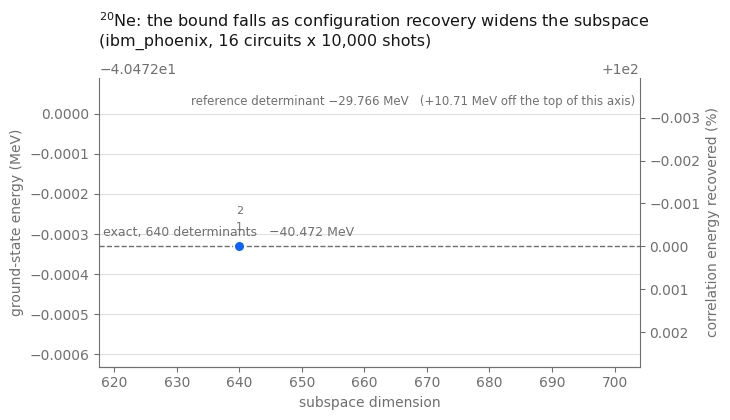
**対角化は変分上界を与えます。**各反復の部分空間は前のものを含むため、エネルギーの列は単調に下がり、その各要素は、それを生んだサンプルのノイズにかかわらず、真の基底状態エネルギーに対する厳密な上界です。
result_sd = recovery_loop(
    inter_sd,
    sp_sd,
    matrix_sd,
    probs_sd,
    occ_sd,
    N_PROTONS,
    N_NEUTRONS,
    max_iterations=4,
    max_dimension=MAX_DIMENSION,
    seed=42,
)

E_SQD_SD = result_sd["energy"]
recovered_sd = 100 * (E_SQD_SD - E_REF_SD) / (E_EXACT_SD - E_REF_SD)

print(f"\nreference determinant   {E_REF_SD:11.6f} MeV")
print(
    f"pooled SQD upper bound         {E_SQD_SD:11.6f} MeV   "
    f"(subspace dimension {len(result_sd['basis'])} of {len(basis_exact_sd)})"
)
print(f"exact diagonalization   {E_EXACT_SD:11.6f} MeV")
print(f"\ncorrelation energy recovered: {recovered_sd:.1f}%")

energies_sd = [h["energy"] for h in result_sd["history"]]
if any(b > a + 1e-9 for a, b in zip(energies_sd, energies_sd[1:])):
    raise AssertionError(
        "the subspaces are not nested; the bound should never rise"
    )
if E_SQD_SD < E_EXACT_SD - 1e-7:
    raise AssertionError(
        f"pooled SQD returned {E_SQD_SD:.6f}, below the exact {E_EXACT_SD:.6f}; "
        "a subspace bound cannot beat the full diagonalization"
    )
iteration 1: 66 proton x 66 neutron halves -> dimension 640, E = -40.472331 MeV
  iteration 2: 66 proton x 66 neutron halves -> dimension 640, E = -40.472331 MeV

reference determinant    -29.765549 MeV
pooled SQD upper bound          -40.472331 MeV   (subspace dimension 640 of 640)
exact diagonalization    -40.472331 MeV

correlation energy recovered: 100.0%
結果を評価する
次のチェックを使って、これらの設定でHeronクラスのバックエンドでの結果を評価します。
-
2つの核子数に関するショット生存率は、陽子数と中性子数が正しいショットの割合を測ります。レジスターが大きくなると低下することがあります。生存率が0に近い場合は、回路の実行に問題がある可能性があります。後処理ではなく、ステップ2のISA深さとバックエンドのキャリブレーションを確認してください。
-
回復ループは、反復ごとに、一定または増加する部分空間の次元と、一定または減少するエネルギーを出力するはずです。反復1ですでに
MAX_DIMENSIONに達している場合、制約となっているのはサンプリングではなく古典的なソルバーです。 -
の回復率は高いはずです。ステップ1で計算したアンザッツの上限が、640個の行列式の空間全体だからです。この実行では、表現力ではなくサンプリングだけが唯一の障害です。
-
前のセルの2つのアサーションは、変分上界を確認します。上界が上がる場合は、部分空間が入れ子でなくなったことを意味し、上界が厳密なエネルギーを下回る場合は、ハードウェアではなくハミルトニアンに問題があることを意味します。
直感に反しますが、よりノイズの多いバックエンドのほうが、クリーンなバックエンドより少し良い上界を与えることがあります。誤りによって、理想的な回路ならサンプルされなかった有効な半分の配置が生じ、変分部分空間を広げても最低固有値は上がらないからです。ノイズ付きシミュレーションでも同じ効果を示せますが、このチュートリアルではハードウェアのサンプルで示します。
# IBM Carbon palette: Blue 60 and Blue 80 for data, Gray 100/70/30 for ink and rules
SURFACE, INK, MUTED, RULE = "#ffffff", "#161616", "#6f6f6f", "#c6c6c6"
SERIES, DEEP, PURPLE = "#0f62fe", "#002d9c", "#6929c4"

def convergence_plot(
    history, e_ref, e_exact, title, colour=SERIES, full_dim=None
):
    """Energy against subspace dimension, scaled to the data rather than to the full window.

    A good run lands within a fraction of a percent of the exact answer, so an axis spanning
    reference-to-exact would squash every point onto one line.  The axis is therefore scaled to
    the data (plus the exact line, when there is one), and the right-hand axis carries the
    fraction of the correlation energy so the absolute and relative readings sit side by side.
    """
    dimensions = [h["dimension"] for h in history]
    energies = [h["energy"] for h in history]

    fig, ax = plt.subplots(figsize=(7.4, 4.3), facecolor=SURFACE)
    ax.set_facecolor(SURFACE)
    ax.plot(
        dimensions,
        energies,
        "-o",
        color=colour,
        linewidth=2,
        markersize=8,
        markeredgecolor=SURFACE,
        markeredgewidth=1.5,
        zorder=3,
    )
    stacked = {}
    for h in history:
        # a converged loop repeats the same point; stack the labels so they do not overprint
        key = (round(h["dimension"]), round(h["energy"], 9))
        offset = 12 + 11 * stacked.get(key, 0)
        stacked[key] = stacked.get(key, 0) + 1
        ax.annotate(
            str(h["iteration"]),
            xy=(h["dimension"], h["energy"]),
            xytext=(0, offset),
            textcoords="offset points",
            ha="center",
            fontsize=8,
            color=MUTED,
        )

    span = (max(dimensions) - min(dimensions)) or max(1, max(dimensions) // 4)
    x_left, x_right = (
        min(dimensions) - 0.14 * span,
        max(dimensions) + 0.40 * span,
    )
    ax.set_xlim(x_left, x_right)

    floor = min(energies) if e_exact is None else min(min(energies), e_exact)
    height = max(max(energies) - floor, 1e-3)
    ax.set_ylim(floor - 0.30 * height, max(energies) + 0.42 * height)

    if e_exact is not None:
        ax.axhline(
            e_exact, color=MUTED, linestyle="--", linewidth=1, zorder=1
        )
        label = "exact" + (f", {full_dim:,} determinants" if full_dim else "")
        ax.annotate(
            f"{label}   {e_exact:.3f} MeV".replace("-", "\u2212"),
            xy=(x_left, e_exact),
            xytext=(3, 5),
            textcoords="offset points",
            ha="left",
            va="bottom",
            color=MUTED,
            fontsize=9,
        )

    # the reference determinant is far off this scale; state it rather than plotting it
    ax.annotate(
        f"reference determinant {e_ref:.3f} MeV".replace("-", "\u2212")
        + f"   ({e_ref - max(energies):+.2f} MeV off the top of this axis)".replace(
            "-", "\u2212"
        ),
        xy=(x_right, max(energies) + 0.42 * height),
        xytext=(-3, -12),
        textcoords="offset points",
        ha="right",
        va="top",
        color=MUTED,
        fontsize=8.5,
    )

    if e_exact is not None and abs(e_exact - e_ref) > 1e-9:
        right = ax.twinx()
        low, high = ax.get_ylim()

        def to_percent(e):
            return 100 * (e - e_ref) / (e_exact - e_ref)

        right.set_ylim(to_percent(low), to_percent(high))
        right.set_ylabel("correlation energy recovered (%)", color=MUTED)
        right.tick_params(colors=MUTED)
        for side in ("top", "left"):
            right.spines[side].set_visible(False)
        right.spines["right"].set_color(MUTED)
        right.spines["bottom"].set_color(MUTED)

    ax.set_xlabel("subspace dimension", color=MUTED)
    ax.set_ylabel("ground-state energy (MeV)", color=MUTED)
    ax.set_title(title, color=INK, fontsize=11.5, loc="left", pad=12)
    ax.grid(axis="y", color=RULE, alpha=0.55)
    ax.tick_params(colors=MUTED)
    for side in ("top", "right"):
        ax.spines[side].set_visible(False)
    for side in ("bottom", "left"):
        ax.spines[side].set_color(MUTED)
    fig.tight_layout()
    return fig

convergence_plot(
    result_sd["history"],
    E_REF_SD,
    E_EXACT_SD,
    f"$^{{20}}$Ne: the bound falls as configuration recovery widens the subspace\n"
    f"({backend.name}, {N_CIRCUITS} circuits x {SHOTS:,} shots)",
    full_dim=len(basis_exact_sd),
)
plt.show()
大規模ハードウェアの例
スケールアップで変わるのは入力だけなので、次に4つのステージを1つの関数にまとめ、コアの上の殻にある40量子ビットのレジスターで、GXPF1相互作用 [3]を使って2回実行します。
2つの実行は、スケーリングの異なる側面を示します。
-
は、2つの価陽子と2つの価中性子を持ち、基底は4,000個の行列式です。レジスターは40量子ビットですが、問題はノートPCでも厳密に対角化できる小ささなので、レジスターサイズを増やした後でも、ハードウェアの結果を厳密な参照値と比較できます。
-
は、4つの価陽子と4つの価中性子を持ち、同じ40量子ビットで対称性が許す行列式が1,963,461個あります。このチュートリアルの密なソルバーはその空間全体を対角化できないため、実行は厳密な上界と、それが改善する参照行列式を返します。
2つの実行にわたって、2つの量に注目してください。固定されたゲート予算に収まるプールの割合は、プールが大きくなるにつれて小さくなり、pack_ensembleはどれだけが含まれるかを報告します。部分空間は、サンプリングで制限されなくなり、ここでの密な古典ソルバーが構築できる最大の行列であるMAX_DIMENSIONで制限されるようになります。この規模では、実運用の計算には選択的配置間相互作用(selected-CI)ソルバーを使います。
ステップ1〜4を組み合わせる
次の関数は、ウォークスルーと同じ順序で、同じステージを呼び出します。
def sqd_run(snt_file, n_protons, n_neutrons, name, exact=True):
    """The whole workflow for one nucleus.  Returns a record of every stage."""
    # -------------------------Step 1-------------------------
    ms = read_snt(DATA / snt_file, n_protons, n_neutrons)
    sp = m_scheme_states(ms)
    inter = Interaction(ms, sp)
    if sum(1 for s in sp if s.tz == -1) * 2 != len(sp):
        raise ValueError(
            f"{name}: post-selection needs equal proton and neutron state counts"
        )
    reference = reference_determinant(sp, inter, n_protons, n_neutrons)
    e_ref = matrix_element(inter, reference, reference)

    raw = excitation_pool(sp, reference)
    ranked = rank_pool(
        inter, reference, [op for op in raw if conserves_symmetry(sp, op)]
    )
    print(
        f"{name}: {len(sp)} qubits, {n_protons}p + {n_neutrons}n, A = {ms.mass_number}"
    )
    print(
        f"  2p2h pool {len(raw)} raw -> {len(ranked)} symmetry-allowed; "
        f"reference energy {e_ref:.6f} MeV"
    )

    # -------------------------Step 2-------------------------
    costs = excitation_costs(len(sp), ranked, costing_manager)
    circuits, bins, isa = pack_to_budget(
        len(sp),
        reference,
        ranked,
        costs,
        DEPTH_BUDGET,
        N_CIRCUITS,
        pass_manager,
    )
    packed = sum(len(b) for b in bins)
    worst = max(two_qubit_depth(c) for c in isa)
    worst_count = max(two_qubit_count(c) for c in isa)
    print(
        f"  packed {packed} of {len(ranked)} excitations; worst circuit two-qubit depth "
        f"{worst}, {worst_count} two-qubit gates"
    )

    # -------------------------Step 3-------------------------
    # a unique tag per run, so the jobs are findable later
    bit_arrays = sample(isa, SHOTS, JOB_TAGS + [name])
    matrix, probabilities, shots = pool_samples(bit_arrays, sp)
    survival = float(
        probabilities[
            (matrix[:, len(sp) // 2 :].sum(axis=1) == n_protons)
            & (matrix[:, : len(sp) // 2].sum(axis=1) == n_neutrons)
        ].sum()
    )
    print(
        f"  {shots:,} shots -> {len(matrix):,} distinct bitstrings, "
        f"{survival:.1%} of shots with the right nucleon numbers"
    )
    if survival == 0.0:
        raise RuntimeError(
            f"{name}: no shot carried the right nucleon numbers"
        )

    # -------------------------Step 4-------------------------
    result = recovery_loop(
        inter,
        sp,
        matrix,
        probabilities,
        reference,
        n_protons,
        n_neutrons,
        max_iterations=4,
        max_dimension=MAX_DIMENSION,
        seed=42,
    )
    energy = result["energy"]

    full_dim = count_basis(sp, n_protons, n_neutrons)  # cheap, even when huge
    e_exact = None
    if exact:
        full = full_basis(sp, n_protons, n_neutrons)
        if len(full) != full_dim:
            raise AssertionError(
                f"{name}: counted {full_dim} determinants but enumerated "
                f"{len(full)}"
            )
        e_exact, _ = ground_state(inter, full)

    print(f"  reference {e_ref:11.6f} MeV     pooled SQD {energy:11.6f} MeV")
    if e_exact is not None:
        print(
            f"  exact     {e_exact:11.6f} MeV  (dimension {full_dim})  ->  "
            f"{100 * (energy - e_ref) / (e_exact - e_ref):.1f}% of the correlation energy"
        )
        if energy < e_exact - 1e-7:
            raise AssertionError(
                f"{name}: pooled SQD bound is below the exact energy"
            )
    else:
        print(
            f"  no exact reference: the symmetry-allowed basis is {full_dim:,} determinants"
        )
        print(
            f"  the bound captures {energy - e_ref:.6f} MeV of correlation energy"
        )
    print()

    return dict(
        name=name,
        qubits=len(sp),
        pool=len(ranked),
        packed=packed,
        two_qubit=worst,
        two_qubit_gates=worst_count,
        shots=shots,
        distinct=len(matrix),
        survival=survival,
        dimension=len(result["basis"]),
        full_dim=full_dim,
        e_ref=e_ref,
        e_sqd=energy,
        e_exact=e_exact,
        history=result["history"],
        # the subspace and its eigenvector cannot be reconstructed from the summary --
        # they depend on the sampled shots -- so keep them for the scaling analysis
        interaction=inter,
        states=sp,
        reference=reference,
        ranked=ranked,
        basis=result["basis"],
        vector=result["vector"],
    )

pretty = {"20Ne": "$^{20}$Ne", "44Ti": "$^{44}$Ti", "48Cr": "$^{48}$Cr"}

small_scale = dict(
    name="20Ne",
    qubits=len(sp_sd),
    pool=len(ranked_sd),
    packed=PACKED_SD,
    two_qubit=worst_sd,
    two_qubit_gates=worst_count_sd,
    shots=shots_sd,
    distinct=len(matrix_sd),
    survival=shot_survival_sd,
    dimension=len(result_sd["basis"]),
    full_dim=len(basis_exact_sd),
    e_ref=E_REF_SD,
    e_sqd=E_SQD_SD,
    e_exact=E_EXACT_SD,
    history=result_sd["history"],
    interaction=inter_sd,
    states=sp_sd,
    reference=occ_sd,
    ranked=ranked_sd,
    basis=result_sd["basis"],
    vector=result_sd["vector"],
)
: 40量子ビットのレジスターでの同じワークフロー
の上の殻には、粒子種ごとに4つの軌道があり、それぞれに20個の磁気副準位があるため、レジスターは40量子ビットです。2つの価陽子と2つの価中性子でになり、対称性が許す行列式は4,000個です — の基底の約6倍で、24量子ビットではなく40量子ビットを使います。
これは、ノートブックが厳密に解ける2つの例のうち大きいほうなので、ハードウェアの結果を厳密な参照値と比較できます。
large_scale_verified = sqd_run("gxpf1.snt", 2, 2, "44Ti", exact=True)
44Ti: 40 qubits, 2p + 2n, A = 44
  2p2h pool 1602 raw -> 174 symmetry-allowed; reference energy -44.309387 MeV
  packed 96 of 174 excitations; worst circuit two-qubit depth 272, 285 two-qubit gates
job dap31a02fm4c73f67dp0: 16 circuits x 10,000 shots on ibm_phoenix
  160,000 shots -> 48,170 distinct bitstrings, 18.6% of shots with the right nucleon numbers
  iteration 1: 187 proton x 189 neutron halves -> dimension 3891, E = -47.849086 MeV
  iteration 2: 190 proton x 190 neutron halves -> dimension 4000, E = -47.876666 MeV
  iteration 3: 190 proton x 190 neutron halves -> dimension 4000, E = -47.876666 MeV
  reference  -44.309387 MeV     pooled SQD  -47.876666 MeV
  exact      -47.876666 MeV  (dimension 4000)  ->  100.0% of the correlation energy
: チュートリアルの厳密対角化の能力を超える
2つの陽子と2つの中性子を追加しても、同じ40量子ビットのレジスター(では4, 4)を使い、基底サイズは約491倍に増えて、対称性が許す行列式は1,963,461個になります。その行列は、このチュートリアルが構築できるものをはるかに超えているため、exact=Falseです。厳密な参照エネルギーはなく、変分上界と、それが改善する参照行列式だけがあります。
このスケールでは2つの点が変わり、どちらも出力から確認できます。プールは数百個の許容励起にまで拡大するため、固定されたゲート予算はプール全体ではなく、その一部しかカバーしません。また、サンプルが張る積部分空間が MAX_DIMENSION より大きくなるため、密行列ソルバーはサンプリングされた重みに基づいてそれを切り詰めます。この上界は依然として厳密ですが、サンプリングされたすべての配置から計算した上界よりも精度が低くなる場合があります。実運用の計算では、サンプルを保持し、より大きな部分空間をサポートするソルバーを使用することになります。
large_scale_unverified = sqd_run("gxpf1.snt", 4, 4, "48Cr", exact=False)
48Cr: 40 qubits, 4p + 4n, A = 48
  2p2h pool 5536 raw -> 582 symmetry-allowed; reference energy -93.041237 MeV
  packed 96 of 582 excitations; worst circuit two-qubit depth 224, 279 two-qubit gates
job dap32a02fm4c73f67eog: 16 circuits x 10,000 shots on ibm_phoenix
  160,000 shots -> 55,436 distinct bitstrings, 18.6% of shots with the right nucleon numbers
  iteration 1: 223 proton x 223 neutron halves -> dimension 3977, E = -96.481598 MeV
  iteration 2: 223 proton x 223 neutron halves -> dimension 3977, E = -96.481598 MeV
  reference  -93.041237 MeV     pooled SQD  -96.481598 MeV
  no exact reference: the symmetry-allowed basis is 1,963,461 determinants
  the bound captures -3.440361 MeV of correlation energy
厳密な参照値なしで結果を評価する
の実行には、このチュートリアル内に厳密な参照値がありません。追加のQPU時間や全空間の対角化を使わずに、既存のサンプルを用いて収束を評価し、古典的な選択ベースラインと比較します。
収束しているか? 保持された行列式を、収束した固有ベクトルにおける重みの順に並べ替えると、部分空間は入れ子になります。そのため、 の系列に対して先頭の ブロックを対角化すると、部分空間サイズ2桁分にわたる上界の減少を追跡できます。最大の でもまだ急激に下降している場合は、古典ソルバーの次元上限が律速であり、増やすべきパラメータは MAX_DIMENSION です。平坦になっている場合は、保持された行列式をさらに追加してもほとんど改善せず、さらに進めるには追加の配置をサンプリングする必要があるかもしれません。ハミルトニアンはフルサイズで一度だけ構築され、各段はその主ブロックなので、スイープ全体のコストは段ごとではなく行列構築1回分で済みます。
量子サンプリングは古典的な選択とどう比較されますか? 古典的な選択手順で選んだ同じサイズの部分空間と比較します。摂動論でスコア順にランク付けしたプールを取り、積部分空間を同じ次元まで拡大し、代わりにそれを対角化します。どちらの曲線も同じハミルトニアンに対する厳密な上界なので、同じ次元でより低い方が、より良い行列式を選んだことになります。この比較により、ハードウェアサンプリングがこの古典的ベースランに対してエネルギー推定を改善するかどうかが決まります。
この部分空間は励起状態向けに選択されたものではありません。配置回復は基底状態の占有数を用いて部分空間を誘導するため、高い固有値は最低固有値よりもはるかに収束から遠く、最初の励起エネルギーは測定された をかなり上回ります。励起状態に適切に到達するには、それらのために選択された部分空間が必要です。
def subspace_scaling(
    inter, basis, vector, points=18, smallest=32, largest=None
):
    """Nested Rayleigh-Ritz sweep: the lowest eigenvalue of the leading d x d block, for a ladder of d.

    Reordering the basis by descending weight in the converged eigenvector makes every subspace in
    the ladder a subset of the next, so the energies fall monotonically and each one is a valid
    variational bound.  H is built once at full size; each rung is a principal block.
    """
    order = np.argsort(-(np.abs(vector) ** 2))
    ordered = [basis[i] for i in order]
    weights = (np.abs(vector) ** 2)[order]
    if (
        largest is not None
    ):  # cap the ladder so two subspaces end at a common dimension
        ordered, weights = ordered[:largest], weights[:largest]
    H = subspace_hamiltonian(inter, ordered)
    dimensions = np.unique(
        np.geomspace(smallest, len(ordered), points).astype(int)
    )
    rows = [
        (
            int(d),
            float(
                eigh(H[:d, :d], eigvals_only=True, subset_by_index=[0, 0])[0]
            ),
        )
        for d in dimensions
    ]
    return rows, np.cumsum(weights)

def classical_selection(
    inter, sp, reference, ranked, target, n_protons, n_neutrons
):
    """The subspace classical perturbative ranking would pick, grown to `target` dimension.

    Same product construction as the sampled subspace, and the same truncation discipline -- half
    configurations are offered to `grow_subspace` in order of importance and it takes as many as
    fit.  The only difference from the sampled path is where the ordering comes from: PT2 score
    here, measured sampling weight there.  So the comparison isolates *which determinants got
    chosen* and nothing else.

    Truncating by any other rule would not be a fair baseline.  Slicing an arbitrarily ordered
    list, for instance, keeps determinants by accident rather than by importance and makes the
    classical subspace look worse than classical selection really is.
    """
    p_ref = tuple(i for i in reference if sp[i].tz == -1)
    n_ref = tuple(i for i in reference if sp[i].tz == +1)
    reached = {reference}
    proton_order, neutron_order = [p_ref], [n_ref]
    seen_p, seen_n = {p_ref}, {n_ref}
    product_budget = 4 * target

    for op, _, _ in ranked:  # ranked is already in descending PT2 score
        h1, h2, v1, v2 = op
        fresh = {
            tuple(sorted(set(d) - {h1, h2} | {v1, v2}))
            for d in reached
            if {h1, h2} <= set(d) and not {v1, v2} & set(d)
        }
        reached |= fresh
        for det in fresh:  # first appearance fixes a half's rank
            half_p = tuple(i for i in det if sp[i].tz == -1)
            half_n = tuple(i for i in det if sp[i].tz == +1)
            if half_p not in seen_p:
                seen_p.add(half_p)
                proton_order.append(half_p)
            if half_n not in seen_n:
                seen_n.add(half_n)
                neutron_order.append(half_n)
        if len(proton_order) * len(neutron_order) > product_budget:
            # Half-configuration products over-count the subspace, because only the
            # symmetry-allowed ones survive `product_subspace`.  Stopping on the product
            # count alone can therefore leave the basis far short of `target`, so check
            # the dimension actually realized and widen the budget if it falls short.
            trial, _, _ = grow_subspace(
                sp,
                [p_ref],
                [n_ref],
                proton_order,
                neutron_order,
                n_protons,
                n_neutrons,
                max_dimension=target,
            )
            if len(trial) >= target:
                break
            product_budget *= 2

    basis, _, _ = grow_subspace(
        sp,
        [p_ref],
        [n_ref],
        proton_order,
        neutron_order,
        n_protons,
        n_neutrons,
        max_dimension=target,
    )
    return basis

run = large_scale_unverified
if "basis" not in run:
    raise RuntimeError(
        "this cell needs the subspace and eigenvector that sqd_run now returns; "
        "re-run the sqd_run definition and the 48Cr cell"
    )

print(
    f"{run['name']}: sweeping nested subspaces of the sampled basis "
    f"(dimension {run['dimension']})"
)
sampled_rows, cumulative = subspace_scaling(
    run["interaction"], run["basis"], run["vector"]
)

print(
    f"{run['name']}: building the classically selected subspace at the same dimension"
)
classical_basis = classical_selection(
    run["interaction"],
    run["states"],
    run["reference"],
    run["ranked"],
    run["dimension"],
    4,
    4,
)
# Both subspaces must be scored at the same dimension.  Symmetry filtering can still leave
# the classical construction short of the target when the ranked pool runs out, so take the
# dimension both actually reach, cap both ladders there, and verify they agree.
common_dim = min(sampled_rows[-1][0], len(classical_basis))
if common_dim < sampled_rows[-1][0]:
    sampled_rows, _ = subspace_scaling(
        run["interaction"], run["basis"], run["vector"], largest=common_dim
    )
classical_rows, _ = subspace_scaling(
    run["interaction"],
    classical_basis,
    ground_state(run["interaction"], classical_basis)[1],
    largest=common_dim,
)
if sampled_rows[-1][0] != classical_rows[-1][0]:
    raise RuntimeError(
        f"comparison dimensions differ: sampled {sampled_rows[-1][0]}, "
        f"classical {classical_rows[-1][0]}"
    )

advantage = sampled_rows[-1][1] - classical_rows[-1][1]
direction = "lower" if advantage < 0 else "higher"
verdict = "beats" if advantage < 0 else "does not beat"
descent = next(
    e for d, e in reversed(sampled_rows) if d <= sampled_rows[-1][0] / 2
)
for fraction in (0.90, 0.99):
    count = int(np.searchsorted(cumulative, fraction) + 1)
    print(
        f"  {fraction:.0%} of the eigenvector norm sits on {count} determinants "
        f"({count / run['full_dim']:.1e} of the {run['full_dim']:,}-determinant space)"
    )
print(
    f"  bound still falling {1000 * (sampled_rows[-1][1] - descent):+.1f} keV "
    f"over the last doubling of dimension"
)
print(
    f"  sampled {sampled_rows[-1][1]:.6f} MeV vs classically selected "
    f"{classical_rows[-1][1]:.6f} MeV at a verified common dimension of "
    f"{classical_rows[-1][0]:,}"
)
print(
    f"  -> the sampled subspace is {abs(advantage) * 1000:.0f} keV {direction}"
)
48Cr: sweeping nested subspaces of the sampled basis (dimension 3977)
48Cr: building the classically selected subspace at the same dimension
  90% of the eigenvector norm sits on 107 determinants (5.4e-05 of the 1,963,461-determinant space)
  99% of the eigenvector norm sits on 593 determinants (3.0e-04 of the 1,963,461-determinant space)
  bound still falling -15.6 keV over the last doubling of dimension
  sampled -96.481598 MeV vs classically selected -95.314510 MeV at a verified common dimension of 3,957
  -> the sampled subspace is 1167 keV lower
fig, axes = plt.subplots(1, 2, figsize=(11.2, 4.0), facecolor=SURFACE)

# left: two nested convergence curves on the same axes
ax = axes[0]
ax.set_facecolor(SURFACE)
ax.plot(
    [d for d, _ in sampled_rows],
    [e for _, e in sampled_rows],
    "-o",
    color=SERIES,
    linewidth=2,
    markersize=5,
    markeredgecolor=SURFACE,
    markeredgewidth=1,
    zorder=4,
    label="sampled on the QPU",
)
ax.plot(
    [d for d, _ in classical_rows],
    [e for _, e in classical_rows],
    "--s",
    color=MUTED,
    linewidth=1.6,
    markersize=4,
    markeredgecolor=SURFACE,
    markeredgewidth=1,
    zorder=3,
    label="classically selected, same size",
)
ax.axhline(run["e_ref"], color=RULE, linestyle=":", linewidth=1.2, zorder=1)
ax.annotate(
    f"reference determinant {run['e_ref']:.2f} MeV".replace("-", "\u2212"),
    xy=(sampled_rows[-1][0], run["e_ref"]),
    xytext=(-2, 4),
    textcoords="offset points",
    ha="right",
    va="bottom",
    color=MUTED,
    fontsize=8,
)

# mark the gap between the two curves at the largest dimension, not either curve alone
edge = sampled_rows[-1][0]
ax.plot(
    [edge, edge],
    [classical_rows[-1][1], sampled_rows[-1][1]],
    "-",
    color=SERIES,
    linewidth=1.0,
    alpha=0.7,
    zorder=2,
)
ax.annotate(
    f"{abs(advantage) * 1000:.0f} keV {direction}\nat equal dimension",
    xy=(edge, 0.5 * (classical_rows[-1][1] + sampled_rows[-1][1])),
    xytext=(-8, 0),
    textcoords="offset points",
    ha="right",
    va="center",
    color=SERIES,
    fontsize=8.5,
)

ax.set_xscale("log")
ax.set_xlim(sampled_rows[0][0] * 0.75, edge * 1.5)
ax.set_xlabel("subspace dimension", color=MUTED)
ax.set_ylabel("variational upper bound (MeV)", color=MUTED)
ax.set_title(
    f"{pretty[run['name']]}: the bound, and the subspace it {verdict}",
    color=INK,
    fontsize=11,
    loc="left",
    pad=10,
)
legend = ax.legend(frameon=False, fontsize=8.5, loc="lower left")
for text in legend.get_texts():
    text.set_color(MUTED)

# right: why a few thousand determinants can bound two million
ax = axes[1]
ax.set_facecolor(SURFACE)
ranks = np.arange(1, len(cumulative) + 1)
ax.plot(ranks, 100 * cumulative, "-", color=DEEP, linewidth=2, zorder=3)
for fraction, style, label_y in ((0.90, ":", 46), (0.99, "--", 24)):
    count = int(np.searchsorted(cumulative, fraction) + 1)
    ax.axvline(count, color=MUTED, linestyle=style, linewidth=1, zorder=1)
    ax.annotate(
        f"{fraction:.0%} of the norm\non {count} determinants",
        xy=(count, label_y),
        xytext=(7, 0),
        textcoords="offset points",
        ha="left",
        va="center",
        color=MUTED,
        fontsize=8.5,
    )
ax.set_xscale("log")
ax.set_xlim(0.8, len(cumulative) * 2.6)
ax.set_ylim(0, 104)
ax.set_xlabel("determinants, ordered by weight", color=MUTED)
ax.set_ylabel("cumulative share of the eigenvector (%)", color=MUTED)
ax.set_title(
    f"Sparsity: {run['full_dim']:,} determinants in the sector",
    color=INK,
    fontsize=11,
    loc="left",
    pad=10,
)

for ax in axes:
    ax.grid(axis="y", color=RULE, alpha=0.55)
    ax.tick_params(colors=MUTED, labelsize=8.5)
    for side in ("top", "right"):
        ax.spines[side].set_visible(False)
    for side in ("bottom", "left"):
        ax.spines[side].set_color(MUTED)
fig.tight_layout()
plt.show()
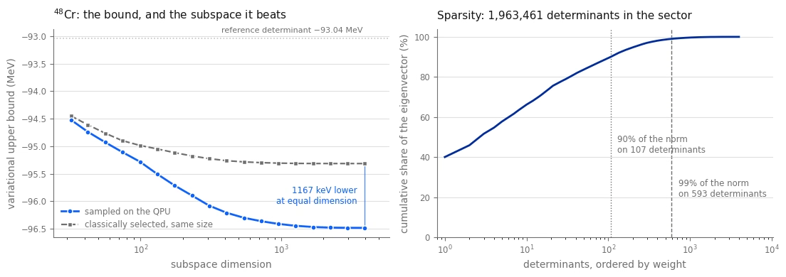
3つの実行を比較する
絶対エネルギーは、異なる原子核や異なる相互作用の間では比較できないため、厳密な参照値が利用できる場合は、各実行で回復された相関エネルギーの割合に注目してください。また、回路の深さと破棄されたショットの割合も比較してください。
runs = [small_scale, large_scale_verified, large_scale_unverified]

print(
    f"{'run':>6}  {'qubits':>6}  {'pool':>9}  {'2q depth':>8}  {'2q gates':>8}  "
    f"{'shots kept':>10}  {'dim':>6}  {'of':>9}  {'% corr':>7}"
)
for r in runs:
    fraction = (
        "--"
        if r["e_exact"] is None
        else f"{100 * (r['e_sqd'] - r['e_ref']) / (r['e_exact'] - r['e_ref']):.1f}%"
    )
    coverage = "{}/{}".format(r["packed"], r["pool"])
    print(
        f"{r['name']:>6}  {r['qubits']:>6}  {coverage:>9}  "
        f"{r['two_qubit']:>8}  {r['two_qubit_gates']:>8}  {r['survival']:>9.1%}  "
        f"{r['dimension']:>6}  {(r['full_dim'] or 0):>9,}  {fraction:>7}"
    )

print()
for r in runs:
    exact = (
        f"exact {r['e_exact']:11.6f}"
        if r["e_exact"] is not None
        else "exact  unavailable"
    )
    print(
        f"{r['name']:>6}   reference {r['e_ref']:11.6f}   pooled SQD {r['e_sqd']:11.6f}   {exact} MeV"
    )
run  qubits       pool  2q depth  2q gates  shots kept     dim         of   % corr
  20Ne      24      78/78       228       234      31.5%     640        640   100.0%
  44Ti      40     96/174       272       285      18.6%    4000      4,000   100.0%
  48Cr      40     96/582       224       279      18.6%    3977  1,963,461       --

  20Ne   reference  -29.765549   pooled SQD  -40.472331   exact  -40.472331 MeV
  44Ti   reference  -44.309387   pooled SQD  -47.876666   exact  -47.876666 MeV
  48Cr   reference  -93.041237   pooled SQD  -96.481598   exact  unavailable MeV
# Left: how much of the correlation energy was recovered, where the exact answer is known.
# Right: the bound itself for the run that has nothing to score against.
scored = [r for r in runs if r["e_exact"] is not None]

fig, ax = plt.subplots(figsize=(6.4, 3.9), facecolor=SURFACE)
ax.set_facecolor(SURFACE)
labels = [
    f"{pretty[r['name']]}\n{r['qubits']} qubits\n{r['full_dim']:,} determinants"
    for r in scored
]
fractions = [
    100 * (r["e_sqd"] - r["e_ref"]) / (r["e_exact"] - r["e_ref"])
    for r in scored
]
shades = [SERIES, DEEP, PURPLE]
bars = ax.bar(
    labels, fractions, width=0.46, color=shades[: len(scored)], zorder=3
)
for bar, fraction, r in zip(bars, fractions, scored):
    ax.annotate(
        f"{fraction:.1f}%",
        xy=(bar.get_x() + bar.get_width() / 2, fraction),
        xytext=(0, 5),
        textcoords="offset points",
        ha="center",
        va="bottom",
        color=INK,
        fontsize=10,
    )
    ax.annotate(
        f"dim {r['dimension']:,}",
        xy=(bar.get_x() + bar.get_width() / 2, 3),
        ha="center",
        va="bottom",
        color=SURFACE,
        fontsize=8.5,
    )
ax.axhline(100, color=MUTED, linestyle="--", linewidth=1, zorder=1)
ax.annotate(
    "exact diagonalization",
    xy=(-0.45, 100),
    xytext=(0, 4),
    textcoords="offset points",
    ha="left",
    va="bottom",
    color=MUTED,
    fontsize=8.5,
)
ax.set_ylim(0, 118)
ax.set_ylabel("correlation energy recovered (%)", color=MUTED)
ax.set_title(
    f"Where the exact answer is known ({backend.name})",
    color=INK,
    fontsize=11,
    loc="left",
    pad=10,
)
ax.grid(axis="y", color=RULE, alpha=0.55)
ax.tick_params(colors=MUTED, labelsize=8.5)
for side in ("top", "right"):
    ax.spines[side].set_visible(False)
for side in ("bottom", "left"):
    ax.spines[side].set_color(MUTED)
fig.tight_layout()
plt.show()

# the same convergence view as the walkthrough, for the run with no exact reference
convergence_plot(
    large_scale_unverified["history"],
    large_scale_unverified["e_ref"],
    None,
    f"{pretty[large_scale_unverified['name']]}: "
    f"{large_scale_unverified['full_dim']:,} determinants, no exact answer to score against\n"
    f"({backend.name}, {N_CIRCUITS} circuits x {SHOTS:,} shots)",
    colour=DEEP,
)
plt.show()

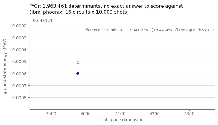
まとめ
入力を除いて変更のない1つのワークフローを、3つの問題サイズでQPU上で実行しました。厳密に確認できる24量子ビットの問題、同じく厳密に確認できる40量子ビットの問題、そしてこのチュートリアルの厳密対角化の能力を超える、200万近い基底状態を持つ40量子ビットの問題です。
3つの実行は、次の点を示しています。
-
量子ステップが行うべきことは行列式の提案だけです。 回路は固定されており、2次摂動論から初期化され、最適化されることはありません。このワークフローでは、振幅が正確である必要はなく、サポートが有用であることだけが求められます。選択された部分空間での古典的対角化は変分上界を与えますが、その上界はサンプリングされた配置によって変動します。
-
量子ビット励起は回路の深さを減らします。 重要なのはサポートだけなので、フェルミオン励起ブロックを量子ビット励起に置き換えることができ、そのコストは接続する軌道間の距離に応じて増加しません。ステップ2では、実際のバックエンドでの削減量を測定しました。これは、コヒーレンス内に余裕をもって収まる回路と、収まらない回路の違いに相当します。
-
配置回復はノイズを含むサンプルを再利用します。 陽子数または中性子数が誤っているすべてのショットは、破棄されるのではなく、現在の占有数の推定値に照らして修復され、修復された各半配置は部分空間に配置を追加できます。変分部分空間を広げても、その最低固有値が上がることはありません。このチュートリアルでは、ハードウェアのサンプルを用いて配置回復を実演します。
-
スケールを上げると律速要因が移り変わります。 24量子ビットでは、アンザッツは厳密解に到達でき、妨げになっていたのはサンプリングだけでした。各核種に4個の価核子を持つ40量子ビットでは、ゲート予算はプールの一部しかカバーせず、密行列の古典ソルバーが部分空間を制限します。3つのうちどれが制約になっているかを見極めることが、このワークフローが教える実践的なスキルです。
次のステップ
次の関連リソースもご覧ください。
-
化学ハミルトニアンのサンプルベース量子対角化: SQDアドオンの選択CIソルバーを使用し、同じアルゴリズムを電子構造に適用します。
-
SQDアドオンのドキュメント: 事後選択、サブサンプリング、配置回復のユーティリティ。
-
量子対角化アルゴリズム: クリロフ変種を含む、部分空間対角化に関する完全なコース。
-
トランスパイルの紹介: 回路が2量子ビットゲートに支配されている場合に重要となる、パスマネージャーのオプション。
-
実行モード: 独立したジョブをスケジューリングするためのbatch modeを紹介します。
検討すべき拡張
-
密行列ソルバーを置き換える。 のスケールでは
MAX_DIMENSIONがすべての上限であり、その理由は密行列に対するnp.linalg.eighにあります。同じ射影ハミルトニアンを疎行列として構築し、scipy.sparse.linalg.eigshなどの反復固有値ソルバー、または核の2体相互作用向けに設計されたDavidsonソルバーや選択CIソルバーを使用すれば、より大きな部分空間をサポートできる可能性があります。実際の限界は行列の疎性、利用可能なメモリ、ソルバーの収束に依存し、このチュートリアルではこの拡張のベンチマークは行いません。SQDアドオンのqiskit_addon_sqd.fermion.solve_sciは、そのまま置き換えられるものではありません。電子構造ソルバーをラップしており、その形式の1体および2体積分を想定しているため、共有された陽子 中性子の積構造だけでは不十分です。これを使うには、式(1)のシェルモデル相互作用をそれらの積分にマッピングし、このノートブックがすでに計算している厳密エネルギーに対して結果を検証する必要があります。 -
バッチ処理とサブサンプリングを追加する。 公開されているプールSQDワークフローは、反復ごとに複数の独立したサブサンプルを対角化し、最良のものを保持します。このチュートリアルでは反復ごとに1バッチを使用しています。これは変分上界には影響しませんが、ショット数を増やすことが有効かどうかを示す分散情報は得られません。
-
励起状態と他のセクター。 各部分空間ハミルトニアンの高い固有値は、同じ対称性セクター内の励起状態に対する上界であり、 で実行すると他のセクターに到達できます。ステップ1の のチェックは、この計算のすでに半分に相当します。
-
殻をまたぐモデル空間。 単一の主殻内ではパリティが自動的に満たされるため、ここでは何の働きもしません。- 空間は のパリティを混合するため、パリティは真の第4の制約となり、SQDのハミング重み修復も積構造も、単独ではこれを捉えられません。
-
奇数質量の原子核。
reference_determinantは各核種の価核子数が偶数であることを必要とします。時間反転対をなす充填が を強制するためです。奇数の原子核には、半整数の 目標と、対をなさない参照が必要です。
付録
このセクションでは、セットアップセクションで導入したヘルパーの背後にある考え方を説明します。
質量依存の再スケーリングが省略できない理由
経験的なシェルモデル相互作用は、ある質量でフィットされ、同位体の系列全体に適用されます。その際、2体行列要素は としてスケールされます。2つの相互作用ファイルはどちらも を持ち、 はUSDファミリーでは 、GXPF1では です。.snt ファイルの2体ヘッダー行では、これら2つの数値が振動子周波数とコアエネルギーが置かれそうな位置にあるため、読み誤りやすくなります。指数を定数のコアエネルギーとして読むと、すべての対角要素に見かけ上のオフセットが加わり、かつ再スケーリングが抜け落ちて、相関エネルギーが数パーセント変わってしまいます。ステップ1の対称性チェックだけでは、エネルギースケールは検証できません。MeV単位で測定した 励起エネルギーを実験値と比較することで、質量依存の再スケーリングに対する追加のチェックが得られます。励起エネルギーはレベル間の差であるため、すべてのエネルギーに加わる定数オフセットは検出できません。
参照を充填ではなく探索で求める理由
最も分かりやすい参照は、最低の1粒子エネルギーを順に充填した行列式です。しかし、これは最低エネルギーの行列式ではありません。式(1)の対角部分には2体項 が含まれ、対相互作用は、利用可能な最大の にある時間反転 のパートナーを占有することを強く好むためです。 殻では、これは の対と の の対の違いに相当し、約1 MeVの差になります。 殻では約2 MeVに近くなります。参照エネルギーは「回復された相関エネルギー」という指標のゼロ点を定義するため、不適切な選択はその指標を水増しし、精度の低い出発点を与えてしまいます。
対をなす充填に限定すると、核種ごとに 個(多くても数千個)の候補しかないため、全探索が安価になり、 も保証されます。このチュートリアルで完全列挙と照合できるすべてのケースにおいて、探索は大域的に最低の対角要素を持つ行列式を返し、それは厳密な基底状態の単一最大成分でもあります。
厳密な2準位の角度ではなく1次の振幅を使う理由
空間 で ハミルトニアンを対角化すると、混合角 が得られます。これを孤立した2準位に対する正しい選択と呼びたくなるかもしれません。このアンザッツでは、数十個の励起ブロックが同じ参照に対して順次作用するため、各ブロックを個別に最適化しても、合成回路が最適になるとは限りません。
角度の選択は、回路の役割によって決まります。すべての実数 に対して が成り立つため、厳密な角度は常に1次の振幅 より大きさが小さく、したがって参照行列式に常により多くの振幅を残します。参照により多くの振幅を残す回路は、参照をより頻繁に返し、異なる励起行列式を返す頻度は低くなります。プールSQDでは、ショットの有用な出力は古典ステップがまだ見ていない行列式であるため、このチュートリアルではより大きな角度を使用します。古典的対角化は回路の振幅を完全に破棄して独自に導出し直すため、どちらの角度も正確である必要はありません。
プールSQDが量子ビット励起を使える理由
フェルミオン励起 は、Jordan-Wigner変換により8個のパウリ列に写像され、それぞれが最も外側の添字の間にあるすべての量子ビットに 演算子を持ちます。これらの列はフェルミオンの符号を符号化しており、そのコストはスパンとともに増加します。陽子-中性子励起の場合、スパンはレジスタ全体です。
これらを取り除くと、Yordanovらの量子ビット励起演算子 [5] が得られます。これは別の演算子であり、それが準備する状態は、振幅の符号においてフェルミオンのものと異なり、2つのサンプリング分布は大きく異なる場合があります。変わらないのは、どの行列式が非零の振幅を持つかという点です。各ブロックは、作用するすべての行列式 について、依然として同じ2次元空間 内で回転し、両方の核子数、、パリティを厳密に保存するためです。したがって、到達可能な行列式の集合は同一であり、プールSQDが使用するのはこの到達可能集合だけです。古典的対角化は、いずれにせよ独自の振幅を割り当てます。ステップ2では、プールからの実際の演算子で同一サポートの主張を検証し、この置き換えによる削減量を測定します。
制約として、サンプリングの重みは異なるため、2つの構成は有限のショット数では同じ順序で行列式を発見するとは限りません。回路に入れる励起を決めるランキングは古典的で変わらず、古典ステップはいずれにせよすべてを再重み付けするため、サンプリング重みの違いは、回路の深さを減らすためのトレードオフです。
が積ステージに属する理由
事後選択と配置回復はどちらもハミング重みに作用します。つまり、レジスタの片方の半分にある陽子数と、もう片方の半分にある中性子数です。 はその形ではありません。これは、陽子配置と中性子配置を組み合わせたものの性質です。陽子半分と中性子半分がそれぞれ正しい核子数を持つショットは、たとえそれらの 値が打ち消し合わなくても、2つの使用可能な半配置を含んでいます。 の陽子半分は、 の中性子半分と組み合わされれば、まったく問題ないからです。全体の でショット全体をフィルタリングすると両方の半分が捨てられてしまいますが、再結合された積に を課せば、それらを残せます。同じ議論により、このケースで recover_configurations が有用であるために の概念を必要としない理由も説明されます。
参考文献
-
J. Robledo-Moreno, M. Motta, H. Haas, et al., "Chemistry beyond the scale of exact diagonalization on a quantum-centric supercomputer", Science Advances 11, eadu9991 (2025). arXiv:2405.05068
-
B. A. Brown and W. A. Richter, "New USD Hamiltonians for the sd shell", Physical Review C 74, 034315 (2006). 組み込みの
usda.sntファイルは、W. A. Richter, S. Mkhize and B. A. Brown, "sd-shell observables for the USDA and USDB Hamiltonians", Physical Review C 78, 064302 (2008) に表としてまとめられたUSDAパラメータを保持しています。 -
M. Honma, T. Otsuka, B. A. Brown and T. Mizusaki, "Effective interaction for pf-shell nuclei", Physical Review C 65, 061301(R) (2002).
-
B. Huron, J. P. Malrieu and P. Rancurel, "Iterative perturbation calculations of ground and excited state energies from multiconfigurational zeroth-order wavefunctions", The Journal of Chemical Physics 58, 5745 (1973).
-
Y. S. Yordanov, D. R. M. Arvidsson-Shukur and C. H. W. Barnes, "Efficient quantum circuits for quantum computational chemistry", Physical Review A 102, 062612 (2020).
-
National Nuclear Data Center, Evaluated Nuclear Structure Data File, Brookhaven National Laboratory. ステップ1で引用した、測定された 励起エネルギーの出典です。