Samplexの入力と出力

はじめに

Samplex は、samplomaticライブラリのコア・タイプです。samplexは、あるテンプレート回路のパラメーターに対するパラメトリックな確率分布を表し、バインドされたテンプレート回路の実行で収集したデータの後処理に使う、配列値の他のフィールドも持ちます。中心となるインターフェースは sample() メソッドで、この分布から抽出して配列の集合を生成します。

このガイドでは、sample() インターフェースの使い方、必要な入力の照会と指定の方法、期待される出力の確認方法を説明します。sample() に渡される配列および返される配列は、厳密に型付けされています。つまり、samplexのインスタンスについて、それらの名前、型、形状は固定されており、サンプリングを行う前に照会できます。samplexに存在する入力と出力は、多くの要因に依存します。たとえば、測定ツワーリングの有無や、ノイズ注入が必要かどうかなどです。このため、一般に、2つのsamplexインスタンスが同じ入力と出力を持つことは想定されていません。

セットアップ

まず、ボックス化された回路を構築し、それをsamplexとテンプレートのペアにビルドします。これらは以降の例で使用します。回路を手動でボックス化する際、このガイドでは alpha、beta、ref1、ref2、mod_ref1、mod_ref2、mod_ref3、conclude という名前を使用することに注意してください。さらに、この回路には4つの Parameter オブジェクトがあります。このガイドでは、これらがそれぞれsamplexの入力と出力でどのような役割を果たすかを示します。回路を自動的にボックス化する方法については、トランスパイラー・ガイドを参照してください。

import matplotlib.pyplot as plt
import numpy as np
from qiskit.circuit import ClassicalRegister, Parameter, QuantumCircuit, QuantumRegister
from qiskit.quantum_info import Operator, Pauli, PauliLindbladMap

from samplomatic import ChangeBasis, InjectNoise, Twirl, build

# our circuit has two classical registers named alpha and beta
circuit = QuantumCircuit(
    QuantumRegister(4), alpha := ClassicalRegister(3, "alpha"), beta := ClassicalRegister(1, "beta")
)

# the first box is only twirled
with circuit.box([Twirl()]):
    for idx in range(4):
        circuit.rx(Parameter(f"a{idx}"), idx)
    circuit.cz(0, 1)
    circuit.cz(1, 2)

# the second box is twirled, and has noise injected
with circuit.box([Twirl(), InjectNoise(ref="ref1", modifier_ref="mod_ref1")]):
    circuit.h(1)
    circuit.cz(1, 2)

# the third box is twirled, and has different noise injected
with circuit.box([Twirl(), InjectNoise(ref="ref2", modifier_ref="mod_ref2")]):
    circuit.rx(0.1, range(4))
    circuit.cz(0, 1)
    circuit.cz(1, 2)

# the fourth box is the same as the second, but with a different modifer ref
with circuit.box([Twirl(), InjectNoise(ref="ref1", modifier_ref="mod_ref3")]):
    circuit.h(1)
    circuit.cz(1, 2)

circuit.barrier()

# the final two boxes twirl, and add a basis change in one case
with circuit.box([Twirl(), ChangeBasis(ref="conclude")]):
    circuit.measure(range(3), alpha)

with circuit.box([Twirl()]):
    circuit.measure([3], beta)

circuit.draw("mpl")

次に、ボックス化された回路に対して build() を呼び出し、テンプレートとsamplexのペアを構築します。各ボックスが、ドレッシングを実装する rz-sx-rz-sx-rz フラグメントを含むバリアの「サンドイッチ」に変換される様子が確認できます。

template, samplex = build(circuit)

template.draw("mpl", fold=100)

samplexのDAGをプロットし、ノードにカーソルを合わせて次の内容を確認します。

• すべてのサンプリング・ノード(星)は、ツワーリングのためのランダム化の生成、ノイズ・モデルからのサンプリング、または基底変換の注入を担当します。

• すべてのコレクション・ノード(蝶ネクタイ)は、出力スライス(測定の反転またはパラメーターの角度)のレンダリングを担当します。

• すべての中間ノード(円)は、さまざまな種類のデータ操作を担当します。

samplex.draw()

必要な入力と期待される出力を照会する

必要な入力と期待される出力を確認する最も簡単な方法は、Samplex オブジェクトを表示することです。配列項目は '{name}' <{type}[{shape}...]> の形式で表示され、必須の入力はオプションの入力より前に並びます。

print(samplex)

Samplex(<58 nodes>)
  Inputs:
  - 'basis_changes.conclude' <uint8[3]>: Basis changing gates, in the symplectic ordering
      I=0, Z=1, X=2, and Y=3.
  - 'parameter_values' <float64[4]>: Input parameter values to use during sampling.
  - 'pauli_lindblad_maps.ref1' <PauliLindbladMap>: A PauliLindblad map acting on 2 qubits,
      with 'num_terms_ref1' terms.
  - 'pauli_lindblad_maps.ref2' <PauliLindbladMap>: A PauliLindblad map acting on 4 qubits,
      with 'num_terms_ref2' terms.

  - 'local_scales.mod_ref1' <float64['num_terms_ref1']>: (Optional) An array of factors by
      which to scale individual rates of a Pauli Lindblad map, where the order should match the
      corresponding list of terms.
  - 'local_scales.mod_ref2' <float64['num_terms_ref2']>: (Optional) An array of factors by
      which to scale individual rates of a Pauli Lindblad map, where the order should match the
      corresponding list of terms.
  - 'local_scales.mod_ref3' <float64['num_terms_ref1']>: (Optional) An array of factors by
      which to scale individual rates of a Pauli Lindblad map, where the order should match the
      corresponding list of terms.
  - 'noise_scales.mod_ref1' <float64[]>: (Optional) A scalar factor by which to scale rates
      of a Pauli Lindblad map.
  - 'noise_scales.mod_ref2' <float64[]>: (Optional) A scalar factor by which to scale rates
      of a Pauli Lindblad map.
  - 'noise_scales.mod_ref3' <float64[]>: (Optional) A scalar factor by which to scale rates
      of a Pauli Lindblad map.
  Outputs:
    * 'measurement_flips.alpha' <bool['num_randomizations', 1, 3]>: Bit-flip corrections
        for measurement twirling.
    * 'measurement_flips.beta' <bool['num_randomizations', 1, 1]>: Bit-flip corrections for
        measurement twirling.
    * 'parameter_values' <float32['num_randomizations', 48]>: Parameter values valid for an
        associated template circuit.
    * 'pauli_signs' <bool['num_randomizations', 3]>: Signs from sampled Pauli Lindblad
        maps, where boolean values represent the parity of the number of non-trivial factors in the
        sampled error that arise from negative rates. In other words, in order to implement basic
        PEC, the sign used to correct expectation values should be ``(-1)**bool_value``. The order
        matches the iteration order of boxes in the original circuit with noise injection
        annotations.

samplexの inputs() と outputs() は、名前、形状、型、説明といった詳細情報も含め、プログラムから照会することもできます。これらのメソッドの戻り値の型はどちらも TensorInterface です。たとえば、次のコードは入力インターフェースのすべての仕様を一覧表示します。

samplex.inputs().specs

[TensorSpecification('basis_changes.conclude', (3,), dtype('uint8'), 'Basis changing gates, in the symplectic ordering I=0, Z=1, X=2, and Y=3.'),
 TensorSpecification('local_scales.mod_ref1', ('num_terms_ref1',), dtype('float64'), 'An array of factors by which to scale individual rates of a Pauli Lindblad map, where the order should match the corresponding list of terms.', optional=True),
 TensorSpecification('local_scales.mod_ref2', ('num_terms_ref2',), dtype('float64'), 'An array of factors by which to scale individual rates of a Pauli Lindblad map, where the order should match the corresponding list of terms.', optional=True),
 TensorSpecification('local_scales.mod_ref3', ('num_terms_ref1',), dtype('float64'), 'An array of factors by which to scale individual rates of a Pauli Lindblad map, where the order should match the corresponding list of terms.', optional=True),
 TensorSpecification('noise_scales.mod_ref1', (), dtype('float64'), 'A scalar factor by which to scale rates of a Pauli Lindblad map.', optional=True),
 TensorSpecification('noise_scales.mod_ref2', (), dtype('float64'), 'A scalar factor by which to scale rates of a Pauli Lindblad map.', optional=True),
 TensorSpecification('noise_scales.mod_ref3', (), dtype('float64'), 'A scalar factor by which to scale rates of a Pauli Lindblad map.', optional=True),
 TensorSpecification('parameter_values', (4,), dtype('float64'), 'Input parameter values to use during sampling.'),
 PauliLindbladMapSpecification('pauli_lindblad_maps.ref1', num_qubits=2, num_terms=num_terms_ref1),
 PauliLindbladMapSpecification('pauli_lindblad_maps.ref2', num_qubits=4, num_terms=num_terms_ref2)]

次の例では、名前に文字列 "flips" を含む出力指定子について、いくつかの情報を表示します。

for spec in samplex.outputs().get_specs("flips"):
    print(spec.name, spec.shape, spec.dtype)

measurement_flips.alpha ('num_randomizations', 1, 3) bool
measurement_flips.beta ('num_randomizations', 1, 1) bool

入力値をバインドしてサンプリングする

sample() を行うには、samplexに、少なくとも必須とマークされた inputs() の値が必要です。これらの値はまず入力インターフェースにバインドされ、必要なすべての型チェック(場合によっては型の強制変換)と形状の分析が行われます。型や形状に問題がある場合、または必須の値が欠けている場合は、詳細なエラーが発生します。

入力のバインド

次の例では、必須の入力値が sample() メソッドに渡されます。続いて、それを使ってsamplexから3つのランダム化を抽出します。ドレッシングから必要なバインディングは、ノイズ注入のためのPauli Lindbladマップと基底変換の配列です。さらに、元のボックス化された回路の4つのパラメーターの値が必要で、この場合は np.linspace(0, 1, 4) に設定されています。samplexはこれらのパラメーターをドレッシングに合成するため、実質的にsamplexの出力パラメーター値への修正になります。

inputs = samplex.inputs().bind(
    # bind() concatenates nested dicts with a '.' so that we can
    # set 'pauli_lindblad_maps.noise0/1' as follows. note that the
    # names 'ref1' and 'ref2' derive from the names in the InjectNoise
    # annotation.
    pauli_lindblad_maps={
        "ref1": PauliLindbladMap.identity(2),
        "ref2": PauliLindbladMap.identity(4),
    },
    # likewise, we can set all basis changes as follows, where
    # the name 'conclude' comes from our basis change annotation
    basis_changes={"conclude": [0, 1, 2]},
    # we must provide values for all parameters in the original circuit
    parameter_values=np.linspace(0, 1, 4),
)

outputs = samplex.sample(inputs, num_randomizations=3)
print(outputs)

SamplexOutput(<
  - Dimension constraints: num_randomizations=3

  * 'measurement_flips.alpha' <bool['num_randomizations', 1, 3]>: Bit-flip corrections for
      measurement twirling.
  * 'measurement_flips.beta' <bool['num_randomizations', 1, 1]>: Bit-flip corrections for
      measurement twirling.
  * 'parameter_values' <float32['num_randomizations', 48]>: Parameter values valid for an
      associated template circuit.
  * 'pauli_signs' <bool['num_randomizations', 3]>: Signs from sampled Pauli Lindblad maps,
      where boolean values represent the parity of the number of non-trivial factors in the sampled
      error that arise from negative rates. In other words, in order to implement basic PEC, the
      sign used to correct expectation values should be ``(-1)**bool_value``. The order matches the
      iteration order of boxes in the original circuit with noise injection annotations.
>)

入力は、bind() を複数回呼び出すか、直接の項目代入によって、インターフェースにバインドできます。bind() は利便性のためにネストした辞書形式を受け付けますが、インターフェース自体はフラットなマッピング・オブジェクトであり、通常のマッピングの構文をすべてサポートします。必要な入力がすべて揃うと、fully_bound が真になります。

inputs = (
    samplex.inputs()
    .bind(
        pauli_lindblad_maps={
            "ref1": PauliLindbladMap.identity(2),
            "ref2": PauliLindbladMap.identity(4),
        }
    )
    .bind(parameter_values=np.linspace(0, 1, 4))
)

# once the final requirement is bound, fully_bound becomes True
print("Fully bound?", inputs.fully_bound)
inputs["basis_changes.conclude"] = [0, 2, 3]
print("Fully bound?", inputs.fully_bound)

# setting optional values does not affect whether the interface is fully bound
inputs["noise_scales.mod_ref1"] = 3
print("Fully bound?", inputs.fully_bound)

Fully bound? False
Fully bound? True
Fully bound? True

SamplexOutput サブクラスを含むすべての TensorInterface オブジェクトは、バインドされたデータに対してオブジェクトをマッピングします。つまり、たとえば次のようにしてテンプレートのパラメーター値を取得できます。この場合、3つのランダム化を要求し、テンプレート回路に48個のパラメーターがあるため、形状は (3, 48) になります。

print("(num_randomizations, num_template_params) =", outputs["parameter_values"].shape)
print(outputs["parameter_values"][0, :])

(num_randomizations, num_template_params) = (3, 48)
[ 0.0000000e+00  0.0000000e+00  0.0000000e+00  1.5707964e+00
  3.3333334e-01  1.5707964e+00 -1.5707964e+00  2.4749260e+00
 -1.5707964e+00  1.5707964e+00  1.0000000e+00  1.5707964e+00
  0.0000000e+00  1.5707964e+00  0.0000000e+00  3.1415927e+00
  0.0000000e+00  0.0000000e+00  1.5707964e+00  3.0415926e+00
 -1.5707964e+00 -1.5707964e+00  3.0415926e+00 -1.5707964e+00
 -1.5707964e+00  1.0000000e-01  1.5707964e+00  1.5707964e+00
  1.0000000e-01  1.5707964e+00  3.1415927e+00  1.5707964e+00
  0.0000000e+00  0.0000000e+00  0.0000000e+00  0.0000000e+00
  0.0000000e+00  3.1415927e+00  0.0000000e+00  3.1415927e+00
  0.0000000e+00  0.0000000e+00  3.1415927e+00  1.5707964e+00
  0.0000000e+00  4.4408921e-16  3.1415927e+00  0.0000000e+00]

辞書として入力を指定する

完全にバインドされた TensorInterface を提供する代わりに、下のセルのように、入力を標準的な辞書として指定することもできます。この場合、sample() メソッドは内部で辞書の項目をsamplexの入力インターフェースにバインドし、必要なすべての入力が存在し互換性があることを検証します。

inputs = {
    "pauli_lindblad_maps": {
        "ref1": PauliLindbladMap.identity(2),
        "ref2": PauliLindbladMap.identity(4),
    },
    "basis_changes": {"conclude": [0, 1, 2]},
    "parameter_values": np.linspace(0, 1, 4),
}
outputs = samplex.sample(inputs, num_randomizations=3)

入力の型

現在、インターフェースの値の型は2種類あります。

• 配列値: 形状とデータ型を持ちます。バインドされた値は、可能であればそのデータ型に強制変換されます。任意の次元を自由次元にできます。

• Pauli Lindbladマップ: 型は qiskit.quantum_info.PauliLindbladMap でなければならず、指定された数の量子ビットに作用する必要があります。マップ内の項の数は自由次元です。

# up to precision loss, these are equivalent via automatic type coersion of array inputs
samplex.inputs()["parameter_values"] = [1, 2, 8, 9]
samplex.inputs()["parameter_values"] = np.array([1, 2, 8, 9], dtype=np.float16)

自由次元

TensorInterface クラスには自由次元という概念があります。これは名前付きの整数サイズで、それを制約するデータがインターフェースにバインドされるまで値が決まりません。同じ名前のすべての自由次元は、データをバインドするときに一貫したサイズに解決される必要があり、そうでない場合はエラーが発生します。たとえば、任意のsamplexの outputs() では、ランダム化に対応する配列の軸は、慣例として "num_randomizations" という名前の自由パラメーターです。sample() が呼び出されると、出力に値をバインドします

print("All free dimensions:", outputs.free_dimensions)
print("Current constraints:", outputs.bound_dimensions)

All free dimensions: {'num_randomizations'}
Current constraints: {'num_randomizations': 3}

もう1つの一般的な自由次元のシナリオは、Pauli Lindbladマップの仕様とその修飾子との間で項の制約を共有するものです。qiskit.quantum_info.PauliLindbladMap は項の順序付きシーケンスで、各項には浮動小数点のレートとスパースなPauli表現が含まれます。build() 関数は、各 InjectNoise アノテーションに対して、この型の指定子 "pauli_lindblad_maps.<ref>" を追加し、modifier_ref が含まれている場合は "local_scales.<modifier_ref>" 指定子も追加します。後者は前者のレートとzipしてスケーリングする必要があるため、これらはどちらも、ノイズ・モデルに存在するPauli Lindblad項の数を指定する自由次元 "num_terms_<ref>" を共有します。

# both the PauliLindbladMap and the local scales imply 2 terms, so that the free dimension
# 'num_terms_noise2' is satisfied
inputs = samplex.inputs().bind(
    pauli_lindblad_maps={"ref2": PauliLindbladMap.from_list([("XXYZ", 0.1), ("IIXX", 0.2)])},
    local_scales={"mod_ref2": [1, 2]},
)
print("All free dimensions:", inputs.free_dimensions)
print("Current constraints:", inputs.bound_dimensions)

All free dimensions: {'num_terms_ref1', 'num_terms_ref2'}
Current constraints: {'num_terms_ref2': 2}

量子ビットの順序の規約

build() 関数でボックス化された回路から構築されたSamplexは、sample() への配列値の入力を必要とすることがあり、その1つのインデックスは回路のボックス内の量子ビットに対応します。このセクションでは、そのような軸に使用すべき順序の規約を説明します。要約すると、ボックス化された回路の量子ビットの順序を、そのボックスの量子ビットに限定して使用します。

たとえば、"noise1" に対するPauli Lindbladマップの指定方法を考えるとします。このとき、ノイズ・マップ内の量子ビットの順序は、次の量子ビットを基準にします。

box_of_interest = circuit[1]
qubit_ordering_convention = [qubit for qubit in circuit.qubits if qubit in box_of_interest.qubits]
qubit_ordering_convention

[<Qubit register=(4, "q0"), index=1>, <Qubit register=(4, "q0"), index=2>]

つまり、<Qubit register=(4, "q0"), index=2> に X ノイズを乗せたい場合は、それが qubit_ordering_convention のインデックス 1 にあるため、このようなPauli Lindbladマップを定義する必要があります。

samplex.inputs().bind(
    pauli_lindblad_maps={
        "ref1": (noise1 := PauliLindbladMap.from_sparse_list([("X", [1], 0.12)], num_qubits=2))
    }
)
noise1

<PauliLindbladMap with 1 term on 2 qubits: (0.12)L(X_1)>

基底変換についても同様です。circuit の量子ビット0、1、2を、それぞれ演算子X、Y、Zの+1固有状態に回転させたい場合は、このライブラリ(およびQiskit)で $I=0$、$Z=1$、$X=2$、$Y=3$ という規約が使われていることを踏まえ、次の配列を使用します。

samplex.inputs().bind(basis_changes={"conclude": (basis_change := [2, 3, 1])})
basis_change

[2, 3, 1]

量子ビットの順序の規約は、次のいずれかで定義される順序ではないことに注意してください。

• box_instruction.qubits。ここで box_instruction は、演算が qiskit.circuit.BoxOp である qiskit.circuit.CircuitInstruction です。この量子ビットのリストの順序は、ボックスのコンテキストに命令が追加された順序に依存する可能性があり、紛らわしい規約になってしまうためです。たとえば、with box(): circuit.x([0, 1]) と with box(): circuit.x([1, 0]) では、異なる順序になります。

• box_instruction.operation.body.qubits。これらの量子ビットは外側の回路に現れない場合すらあるためです。BoxOp 命令(または IfElseOp などの他の制御フロー演算)の本体内の量子ビットは、そのスコープ内でのみ一貫した意味を持つことが保証されています。これは定義が不明確な規約となり、一般に使いにくくなります。

テンプレート回路を使ったローカルでのテスト

Samplex が build() 関数を使って構築された場合、出力パラメーター値は、関連するテンプレート回路のパラメーターと直接互換性があるはずです。たとえば、ローカルで確認するために、ランダム化の1つの値をテンプレートにバインドできます。

inputs = samplex.inputs().bind(
    pauli_lindblad_maps={
        "ref1": PauliLindbladMap.identity(2),
        "ref2": PauliLindbladMap.identity(4),
    },
    basis_changes={"conclude": [0, 0, 0]},
    parameter_values=np.linspace(0, 1, 4),
)

outputs = samplex.sample(inputs, num_randomizations=3)

bound_template = template.assign_parameters(outputs["parameter_values"][2])
bound_template.draw("mpl", fold=1000)

これにより、samplexが期待どおりのサンプルを出力していることを検証できます。たとえば、次のコードはバインドされた回路を qiskit.quantum_info.Operator オブジェクトにキャストし、ビット反転のPauliと合成して、3つのランダム化がすべて基本回路と論理的に等価であることを目視で確認します。

from samplomatic.utils import unbox

# Operator requires that we unpack all of the boxes first
unboxed = unbox(circuit).assign_parameters(inputs["parameter_values"])
# We want to plot unitary matrix amplitudes, so we need to remove the non-unitary measurements
unboxed.remove_final_measurements()
unboxed_unitary = Operator(unboxed)

# Plot magnitudes of the unitary matrix represenation of the circuit
plt.subplot(1, 4, 1)
plt.imshow(np.abs(unboxed_unitary))
plt.title("Base Circuit")

# For each randomization we sampled, plot the unitary matrix representation
for idx in range(3):
    bound_template = template.assign_parameters(outputs["parameter_values"][idx])
    bound_template.remove_final_measurements()

    # The example does measurement twirling by compiling random bitflip gates before the
    # measurements, so we need to undo these at the operator level for each randomization.
    # We do this by casting them to Paulis and composing with the bound circuit's unitary
    alpha_flips = Pauli(([0, 0, 0], outputs["measurement_flips.alpha"][idx, 0]))
    beta_flips = Pauli(([0], outputs["measurement_flips.beta"][idx, 0]))
    flips = beta_flips ^ alpha_flips
    bound_unitary = Operator(bound_template) & flips

    # Plot magnitudes of the unitary matrix represenation of the circuit
    plt.subplot(1, 4, idx + 2)
    plt.imshow(np.abs(bound_unitary))
    plt.title(f"Randomization {idx}")

plt.tight_layout()

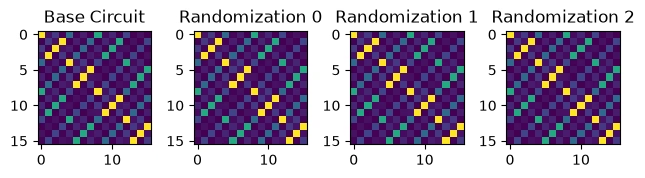
同様に、次のコードは出力パラメーター値とテンプレートをsamplerに渡し、すべてのランダム化について10,000ショットをシミュレートして、得られた期待値(alphaレジスターのみ)を基本回路のシミュレーションの期待値と比較します。

from qiskit.primitives import StatevectorEstimator as Estimator
from qiskit.primitives import StatevectorSampler as Sampler
from qiskit.primitives.containers import BitArray

# simulate some expectation values direction from the base circuit
estimator_job = Estimator().run([(unboxed, ["IZII", "IIZI", "IIIZ"])])
evs = estimator_job.result()[0].data["evs"]

# get the sampler data from each randomization, and do bitflip correction
sampler_job = Sampler().run([(template, outputs["parameter_values"])], shots=10_000)
alpha_data = sampler_job.result()[0].data["alpha"]
alpha_data ^= BitArray.from_bool_array(outputs["measurement_flips.alpha"], "little")

# compare the results
print("  EVs from base circuit:", evs)
print("EVs from randomizations:", alpha_data.expectation_values(["ZII", "IZI", "IIZ"]))

  EVs from base circuit: [0.7819611  0.93553883 0.99500417]
EVs from randomizations: [0.789  0.9366 0.995 ]