Qiskit入門
このノートブックでは、QiskitでQuantumGate・量子Circuitをプログラムする方法、Qiskitパターンを使用してシミュレーターや実際の量子コンピューターで実行する方法を学びます。また、情報をエンコードするさまざまな方法を紹介し、最後に量子テレポーテーションのボーナス例で締めくくります。
始める前に
まだの場合は、インストールとセットアップの手順に従ってください。IBM Quantum™ Platformを使用するためのセットアップの手順も含まれます。
量子コンピューターと対話するには、Jupyter開発環境を使用することを推奨します。推奨される追加の可視化サポート('qiskit[visualization]')を必ずインストールしてください。この例の第2部ではmatplotlibパッケージも必要です。
量子コンピューティング全般については、IBM Quantum Learningの量子情報の基礎コースを参照してください。
インポート
# Added by doQumentation — required packages for this notebook
!pip install -q matplotlib numpy qiskit qiskit-aer qiskit-ibm-runtime
# Import necessary modules for this notebook
import time
import qiskit

from qiskit import QuantumCircuit
from qiskit.quantum_info import Statevector
from qiskit.visualization import plot_bloch_multivector, plot_state_qsphere
from qiskit_aer import AerSimulator
from qiskit.quantum_info import SparsePauliOp
from qiskit.transpiler.preset_passmanagers import generate_preset_pass_manager
from qiskit_ibm_runtime import EstimatorV2 as Estimator
from qiskit_ibm_runtime import SamplerV2 as Sampler
from qiskit_ibm_runtime import QiskitRuntimeService
from qiskit.visualization import plot_histogram
print(qiskit.__version__)
2.3.1
ハードウェア上で量子Circuitを実行するには、まずアカウントを設定する必要があります。 以下の手順で設定できます:
- アップグレードされたIBM Quantum® Platformにアクセスします。
- 右上隅(上の画像参照)でAPIトークンを作成し、安全な場所にコピーします。
- 次のセルで
deleteThisAndPasteYourAPIKeyHereをAPIキーに置き換えます。 - 左下隅(上の画像参照)でインスタンスを作成します。オープンプランを選択してください。
- インスタンスが作成されたら、関連するCRNコードをコピーします。インスタンスを確認するには更新が必要な場合があります。
- 以下のセルで
deleteThisAndPasteYourCRNHereをCRNコードに置き換えます。
IBM Cloud®アカウントの設定方法については、このガイドを参照してください。
⚠️ 注意: APIキーは安全なパスワードと同様に取り扱ってください。安全な環境と信頼できない環境の両方でAPIキーを使用する方法については、クラウドセットアップガイドを参照してください。
#your_api_key = "deleteThisAndPasteYourAPIKeyHere"
#your_crn = "deleteThisAndPasteYourCRNHere"

QiskitRuntimeService.save_account(
    channel="ibm_quantum_platform",
    token=your_api_key,
    instance=your_crn,
    overwrite=True
)
1. 量子Gateと量子Circuit
量子Circuitは量子計算のモデルであり、計算は量子Gateの連続で表されます。代表的な量子Gateを見てみましょう。
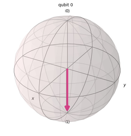
X Gate
X GateはBloch球のX軸周りにラジアン回転させることに相当します。 をに、をにマッピングします。古典コンピューターのNOT Gateの量子版であり、ビットフリップとも呼ばれます。
# Let's apply an X-gate on a |0> qubit
qc = QuantumCircuit(1)
qc.x(0)
qc.draw(output='mpl')

# Let's see Bloch sphere visualization
sv = Statevector(qc)
plot_bloch_multivector(sv)
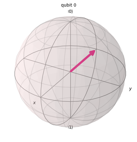
H Gate
アダマールGateは、軸と軸の中間にある軸周りに回転することを表します。
基底状態をにマッピングします。これは測定結果が1または0になる確率が等しい「重ね合わせ」状態を生成することを意味します。この状態はとも書かれます。
# Let's apply an H-gate on a |0> qubit
qc = QuantumCircuit(1)
qc.x(0)
qc.h(0)
qc.draw(output='mpl')

# Let's see Bloch sphere visualization
sv = Statevector(qc)
plot_bloch_multivector(sv)
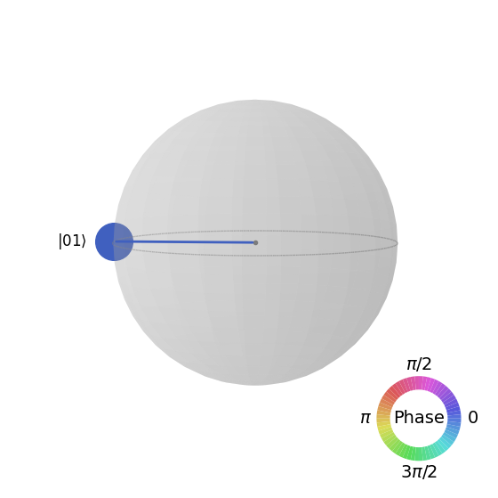
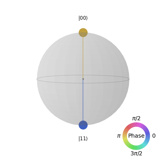
CX Gate(CNOT Gate)
制御NOTゲート(CNOTまたはCX)は2つのqubitに作用します。最初のqubitがのときのみ、2番目のqubitにNOT演算(X Gateを適用するのと同等)を実行し、それ以外の場合は変化させません。注意:Qiskitはビット列の番号を右から左に付けます。
# Let's apply a CX-gate on |11>
qc = QuantumCircuit(2)
qc.x(0)
qc.x(1)
qc.cx(0,1)
qc.draw(output='mpl')

sv=Statevector(qc)
plot_state_qsphere(sv)
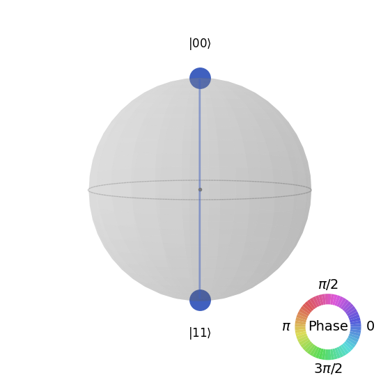
第1ベル状態を作成します
# Create a Bell state circuit

qc = QuantumCircuit(2)
qc.h(0)
qc.cx(0,1)

# Draw the circuit
qc.draw("mpl")

# Plot the state using q-sphere visualization
sv = Statevector(qc)
plot_state_qsphere(sv)
# q-sphere is useful for visualizing states when Bloch sphere fails to
第2ベル状態を作成します
# Create a circuit with the second Bell state

qc = QuantumCircuit(2)
qc.x(0)
qc.h(0)
qc.cx(0,1)

qc.draw("mpl")

説明は以下の通りです:
# Get the statevector of the circuit
sv = Statevector(qc)

# Plot the state using qsphere visualization
plot_state_qsphere(sv)
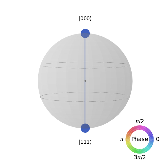
3-qubit GHZ状態を作成します
# Create a circuit with 3-qubit GHZ state

qc= QuantumCircuit(3)
qc.h(0)
qc.cx(0,1)
qc.cx(0,2)

qc.draw("mpl")

# Get the statevector of the circuit
sv = Statevector(qc)

# Plot the state using qsphere visualization
plot_state_qsphere(sv)
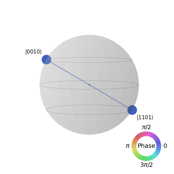
Qiskitロゴ状態を作成します

# Create a circuit with the Qiskit logo state

qc = QuantumCircuit(4)
qc.h(0)
qc.cx(0,1)
qc.cx(0,2)
qc.cx(0,3)
qc.x(1)

# Draw the circuit
qc.draw("mpl")

# Get the statevector of the circuit
sv = Statevector(qc)

# Plot the state using qsphere visualization
plot_state_qsphere(sv)
2. シンプルな量子プログラムの作成と実行
Qiskitパターンを使用して量子プログラムを作成する4つのステップは以下の通りです:
-
問題を量子ネイティブな形式にマッピングする。
-
Circuitと演算子を最適化する。
-
量子プリミティブ関数を使用して実行する。
-
結果を分析する。
2.1 Map the problem to a quantum-native format
量子プログラムにおいて、量子Circuitは量子命令を表現するためのネイティブなフォーマットであり、演算子は測定するオブザーバブルを表します。Circuitを作成する際は、通常、新しいQuantumCircuitオブジェクトを作成し、順番に命令を追加します。
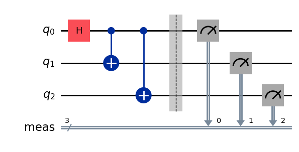
以下のコードセルは、3つのqubitが互いに完全にエンタングルした状態であるGHZ状態を生成するCircuitを作成します。
Qiskit SDKはLSb 0ビット番号付けを使用しており、番目の桁はまたはの値を持ちます。詳細については、Qiskit SDKにおけるビット順序のトピックを参照してください。
# Create a GHZ state circuit

qc = QuantumCircuit(3)
qc.h(0)
qc.cx(0,1)
qc.cx(0,2)
# Draw the circuit
qc.draw("mpl")
利用可能なすべての操作については、ドキュメントのQuantumCircuitを参照してください。
量子Circuitを作成する際は、実行後に返されるデータの種類についても検討する必要があります。Qiskitはデータを返す2つの方法を提供しています。測定対象として選択したqubitの集合に対する確率分布を取得するか、オブザーバブルの期待値を取得するかのいずれかです。Qiskit primitives(ステップ3で詳しく説明)を使用して、これら2つの方法のいずれかでCircuitを測定するようにワークロードを準備してください。
この例では、qiskit.quantum_infoサブモジュールを使用して期待値を測定します。これは演算子(量子状態を変更するアクションやプロセスを表すために使用される数学的オブジェクト)を使用して指定されます。以下のコードセルは、6つの3-qubitパウリ演算子となるZZZ、ZZX、ZII、XXI、ZZI、IIIを作成します。
# Set up six different observables.

observables_labels = ["ZZZ", "ZZX", "ZII", "XXI", "ZZI", "III"]

observables = [SparsePauliOp(label) for label in observables_labels]
print(observables)
[SparsePauliOp(['ZZZ'],
              coeffs=[1.+0.j]), SparsePauliOp(['ZZX'],
              coeffs=[1.+0.j]), SparsePauliOp(['ZII'],
              coeffs=[1.+0.j]), SparsePauliOp(['XXI'],
              coeffs=[1.+0.j]), SparsePauliOp(['ZZI'],
              coeffs=[1.+0.j]), SparsePauliOp(['III'],
              coeffs=[1.+0.j])]
ここで、ZZI演算子のようなものはテンソル積の省略形であり、qubit 2とqubit 1のZを同時に測定し、qubit 2とqubit 1の相関に関する情報を取得することを意味します。このような期待値はとも一般的に表記されます。
観測される状態が3-qubitのGHZ状態である場合、の測定値は1になるはずです。
2.2 Optimize the circuits and operators
デバイス上でCircuitを実行する際は、Circuitに含まれる命令の集合を最適化し、Circuitの全体的な深さ(おおよその命令数)を最小化することが重要です。これにより、エラーとノイズの影響を軽減し、最良の結果を得られるようにします。さらに、Circuitの命令はBackendデバイスの命令セット・アーキテクチャー(ISA)に準拠する必要があり、デバイスの基底Gateおよびqubit接続性を考慮しなければなりません。
以下のコードはジョブを送信する実際のデバイスをインスタンス化し、そのBackendのISAに合わせてCircuitとオブザーバブルを変換します。 事前に認証情報を保存していない場合は、こちらの手順に従ってAPIトークンで認証してください。
# Choose a real backend
service = QiskitRuntimeService(channel='ibm_quantum_platform',)
backend = service.least_busy(min_num_qubits=156)
# print backend details
print(
    f"Name: {backend.name}\n"
    f"Version: {backend.backend_version}\n"
    f"No. of qubits: {backend.num_qubits}\n"
    f"Processor type: {backend.processor_type}\n"
)
Name: ibm_marrakesh
Version: 1.0.21
No. of qubits: 156
Processor type: {'family': 'Heron', 'revision': '2'}
# option to use the AerSimulator instead of a real quantum device
seed_sim=42
backend=AerSimulator.from_backend(backend,seed_simulator=seed_sim)
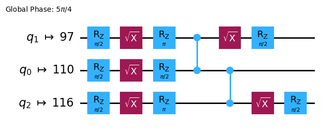
CircuitをISA Circuitにトランスパイルします。
# Convert to an ISA circuit and layout-mapped observables.

pm = generate_preset_pass_manager(backend=backend, optimization_level=2)
isa_circuit = pm.run(qc)

isa_circuit.draw("mpl", idle_wires=False)
mapped_observables = [
    observable.apply_layout(isa_circuit.layout) for observable in observables
]
print(mapped_observables)
[SparsePauliOp(['IIIIIIIIIIIIIIIIZIIIIIZIIIIIIIIIIIIZIIIIIIIIIIIIIIIIIIIIIIIIIIIIIIIIIIIIIIIIIIIIIIIIIIIIIIIIIIIIIIIIIIIIIIIIIIIIIIIIIIIIIIIIIIIIIIIII'],
              coeffs=[1.+0.j]), SparsePauliOp(['IIIIIIIIIIIIIIIIZIIIIIXIIIIIIIIIIIIZIIIIIIIIIIIIIIIIIIIIIIIIIIIIIIIIIIIIIIIIIIIIIIIIIIIIIIIIIIIIIIIIIIIIIIIIIIIIIIIIIIIIIIIIIIIIIIIII'],
              coeffs=[1.+0.j]), SparsePauliOp(['IIIIIIIIIIIIIIIIZIIIIIIIIIIIIIIIIIIIIIIIIIIIIIIIIIIIIIIIIIIIIIIIIIIIIIIIIIIIIIIIIIIIIIIIIIIIIIIIIIIIIIIIIIIIIIIIIIIIIIIIIIIIIIIIIIIII'],
              coeffs=[1.+0.j]), SparsePauliOp(['IIIIIIIIIIIIIIIIXIIIIIIIIIIIIIIIIIIXIIIIIIIIIIIIIIIIIIIIIIIIIIIIIIIIIIIIIIIIIIIIIIIIIIIIIIIIIIIIIIIIIIIIIIIIIIIIIIIIIIIIIIIIIIIIIIIII'],
              coeffs=[1.+0.j]), SparsePauliOp(['IIIIIIIIIIIIIIIIZIIIIIIIIIIIIIIIIIIZIIIIIIIIIIIIIIIIIIIIIIIIIIIIIIIIIIIIIIIIIIIIIIIIIIIIIIIIIIIIIIIIIIIIIIIIIIIIIIIIIIIIIIIIIIIIIIIII'],
              coeffs=[1.+0.j]), SparsePauliOp(['IIIIIIIIIIIIIIIIIIIIIIIIIIIIIIIIIIIIIIIIIIIIIIIIIIIIIIIIIIIIIIIIIIIIIIIIIIIIIIIIIIIIIIIIIIIIIIIIIIIIIIIIIIIIIIIIIIIIIIIIIIIIIIIIIIIII'],
              coeffs=[1.+0.j])]
2.3 Execute using the quantum primitives
量子コンピューターはランダムな結果を生成する可能性があるため、通常はCircuitを何度も実行してサンプルを収集します。Estimatorクラスを使用してオブザーバブルの値を推定できます。Estimatorは2つのprimitivesのうちの一つであり、もう一つは量子コンピューターからデータを取得するために使用できるSamplerです。これらのオブジェクトは、primitive unified bloc(PUB)を使用して、Circuit、オブザーバブル、パラメーター(該当する場合)の選択を実行するrun()メソッドを持っています。
実際の量子ハードウェアでこのコードを実行する場合は、量子コンピューターに固有のノイズを低減するためにエラー軽減・抑制テクニックの適用を検討してください。
# Construct the Estimator instance.
estimator = Estimator(mode=backend)
estimator.options.resilience_level = 1
estimator.options.default_shots = 5000
Estimator primitiveを使用してジョブを送信します。
# One pub, with one circuit to run against six different observables.
job = estimator.run([(isa_circuit, mapped_observables)])

# Use the job ID to retrieve your job data later
print(f">>> Job ID: {job.job_id()}")
>>> Job ID: 97ecd036-1767-49b0-a1dc-c71638c3c3c4
/Users/jma/miniconda3/envs/3122/lib/python3.12/site-packages/qiskit_ibm_runtime/fake_provider/local_service.py:187: UserWarning: The resilience_level option has no effect in local testing mode.
  warnings.warn("The resilience_level option has no effect in local testing mode.")
ジョブの送信後は、現在のPythonインスタンス内でジョブが完了するまで待機するか、job_idを使用して後でデータを取得することができます。(詳細については、ジョブの取得に関するセクションを参照してください。)
ジョブが完了したら、ジョブのresult()属性を通じてその出力を確認します。
# This is the result of the entire submission.  You submitted one Pub,
# so this contains one inner result (and some metadata of its own).
job_result = job.result()

# This is the result from our single pub, which had six observables,
# so contains information on all six.
pub_result = job.result()[0]
次に、Sampler primitiveを使用してCircuitを実行することもできます。
# We include the measurements in the circuit
qc.measure_all()
sampler = Sampler(mode=backend)
qc.draw(output="mpl")
Sampler primitiveを使用してジョブを送信します。
job_sampler = sampler.run(pm.run([qc]))

# Use the job ID to retrieve your job data later
print(f">>> Job ID: {job_sampler.job_id()}")
# Get the results
results_sampler = job_sampler.result()
>>> Job ID: a6ee4d2f-c80d-4a86-9a76-e4b1a74502e7
2.4 Analyze the results
分析ステップは、測定誤差の緩和(Measurement Error Mitigation)やゼロノイズ外挿(ZNE: Zero Noise Extrapolation)などを使って結果を後処理する場合が多いです。これらの結果をさらなる分析のために別のワークフローに渡したり、重要な値やデータのプロットを作成したりすることもあります。一般的に、このステップは解こうとしている問題に固有のものです。この例では、Circuit に対して測定された期待値をそれぞれプロットします。
Estimator に指定したオブザーバブルの期待値と標準偏差は、ジョブ結果の PubResult.data.evs 属性および PubResult.data.stds 属性を通じてアクセスできます。Sampler の結果を取得するには、PubResult.data.meas.get_counts() 関数を使用します。この関数はビット文字列をキー、カウントを対応する値とした dict 形式の測定結果を返します。詳細については、Get started with Sampler を参照してください。
# Plot the result
from matplotlib import pyplot as plt
values = pub_result.data.evs
errors = pub_result.data.stds
# plotting graph
# Plotting with error bars
plt.errorbar(observables_labels, values, yerr=errors, fmt='-o', capsize=5)
plt.xlabel("Observables")
plt.ylabel("Values")
plt.title("Plot of Observables vs Values with Error Bars")
plt.grid(True)
plt.tight_layout()
plt.show()
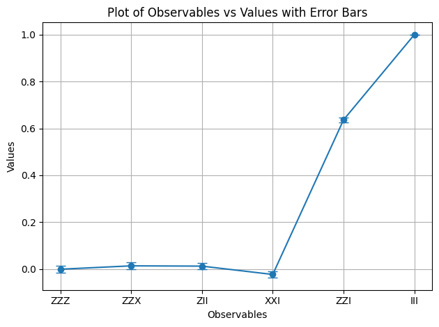
オブザーバブル と の期待値が 1 であることがわかります。 は 2 つのマイナス符号を導入しますが、それらが打ち消し合い、 は恒等演算として作用するため、GHZ 状態が変化しないためです。残りのオブザーバブルの期待値は 0 です。これは、それらの 演算子が奇数個のマイナス符号を導入するか、 演算子が qubit をいくつか反転させて、重なり合う状態が直交するためです。
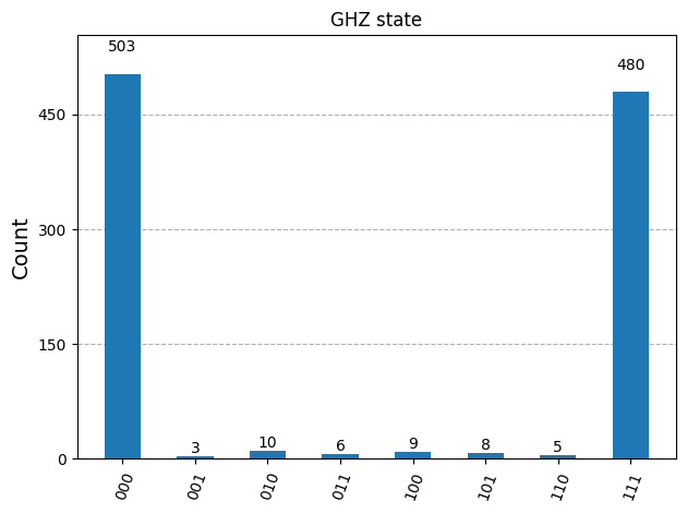
次に、Sampler の結果をプロットします。
counts_list = results_sampler[0].data.meas.get_counts()
print(counts_list)
print(f"Outcomes : {counts_list}")
display(plot_histogram(counts_list, title="GHZ state"))
{'111': 480, '000': 503, '101': 8, '100': 9, '001': 3, '011': 6, '010': 10, '110': 5}
Outcomes : {'111': 480, '000': 503, '101': 8, '100': 9, '001': 3, '011': 6, '010': 10, '110': 5}
2.5 Scale to large numbers of qubits
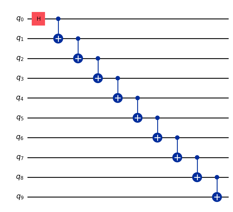
量子コンピューティングにおいて、ユーティリティ・スケールの作業は分野の進歩に不可欠です。そのような作業には、100 qubit を超え、1000 ゲートを超える Circuit を扱うなど、はるかに大規模な計算が必要です。この例では、GHZ 問題を qubit に拡張するという小さな一歩を踏み出します。Qiskit パターンのワークフローを使用し、期待値 を測定して終了します。
Step 1. Map the problem
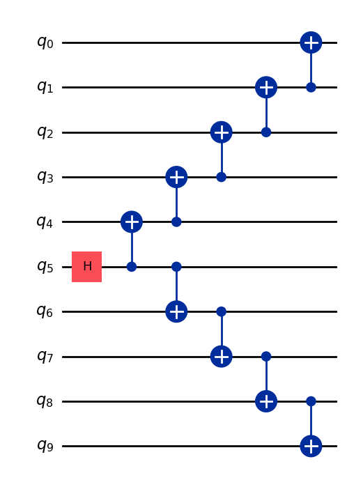
qubit の GHZ 状態(基本的には拡張ベル状態)を準備する QuantumCircuit を返す関数を記述し、その関数を使って 10 qubit の GHZ 状態を準備して、測定するオブザーバブルを収集します。
def get_qc_for_n_qubit_GHZ_state(n: int) -> QuantumCircuit:

    qc = QuantumCircuit(n)
    qc.h(0)
    for i in range(n-1):
        qc.cx(i, i+1)
    return qc
n = 10
qc_n_GHZ = get_qc_for_n_qubit_GHZ_state(n)
qc_n_GHZ.draw("mpl")
次に、対象演算子にマッピングします。この例では、qubit 間の ZZ 演算子を使用して、qubit 同士が離れていくにつれての振る舞いを調べます。離れた qubit 間で期待値が次第に不正確(破損)になることで、存在するノイズのレベルが明らかになります。
# ZZII...II, ZIZI...II, ... , ZIII...IZ
operator_strings = [
    "Z" + i * "I" + "Z" + "I" * (n-i-2) for i in range(n-1)
]
print(operator_strings)
print(len(operator_strings))

operators = [SparsePauliOp(operator) for operator in operator_strings]
['ZZIIIIIIII', 'ZIZIIIIIII', 'ZIIZIIIIII', 'ZIIIZIIIII', 'ZIIIIZIIII', 'ZIIIIIZIII', 'ZIIIIIIZII', 'ZIIIIIIIZI', 'ZIIIIIIIIZ']
9
Step 2. Optimize the problem for execution on quantum backend
Circuit とオブザーバブルを Backend の ISA に合わせて変換します。
# Convert to an ISA circuit and layout-mapped observables.
pm = generate_preset_pass_manager(backend=backend, optimization_level=2)
isa_circuit = pm.run(qc_n_GHZ)
isa_operators_list = [operator.apply_layout(isa_circuit.layout) for operator in operators]
Step 3. Execute on backend
ジョブを送信し、ハードウェア上で実行する場合は、動的デカップリング(Dynamical Decoupling)と呼ばれるエラー低減手法を使ってエラー抑制を有効にします。レジリエンス・レベルは、エラーに対してどの程度の耐性を持たせるかを指定します。レベルが高いほど精度の高い結果が得られますが、処理時間が長くなります。以下のコードで設定されているオプションの詳細については、Configure error mitigation for Qiskit Runtime を参照してください。
# Submit the circuit to Estimator
job = estimator.run([(isa_circuit, isa_operators_list)])
job_id = job.job_id()
/Users/jma/miniconda3/envs/3122/lib/python3.12/site-packages/qiskit_ibm_runtime/fake_provider/local_service.py:187: UserWarning: The resilience_level option has no effect in local testing mode.
  warnings.warn("The resilience_level option has no effect in local testing mode.")
Step 4. Post-process results
実際のハードウェア上でエンタングルした量子状態の振る舞いをより深く理解するために、Z 基底における qubit 間のペアワイズ相関を分析します。具体的には、qubit 0 と各 qubit の相関の強さを測定する期待値 ⟨Z₀Zᵢ⟩ を調べます。特に、以下の値をプロットします。
プロットに表示されると予想される の値はどれですか?
選択肢:
a) が増えるにつれて減少する
b) 1 で一定
c) 1 の周辺で小さなばらつきがある
d) の偶奇で 1 と 0 が交互に現れる
data = list(range(1, len(operators) + 1))  # Distance between the Z operators
result = job.result()[0]
values = result.data.evs  # Expectation value at each Z operator.
values = [
    v / values[0] for v in values
]  # Normalize the expectation values to evaluate how they decay with distance.

plt.plot(data, values, marker="o", label=f"{n}-qubit GHZ state")
plt.xlabel("Distance between qubits $i$")
plt.ylabel(r"$\langle Z_i Z_0 \rangle / \langle Z_1 Z_0 \rangle $")
plt.legend()
plt.show()
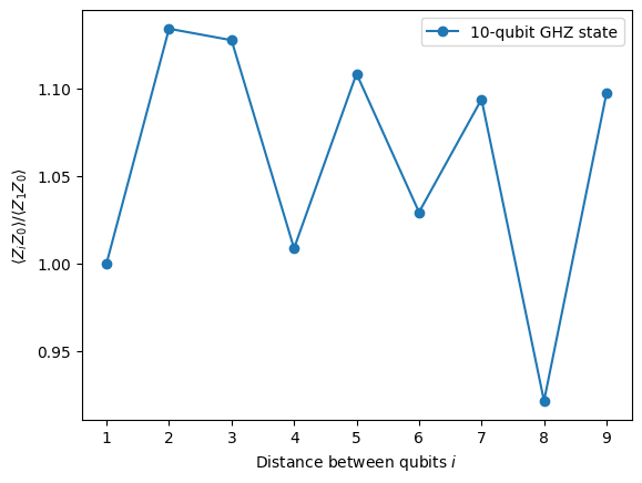
このプロットでは、 が値 1 の周辺で変動していることがわかります。理想的なシミュレーションでは、すべての が 1 になるはずにもかかわらずです。
見てわかるとおり、10 qubit 実験の結果は良好ですが、まだいくらかの誤差があります。結果を改善する 1 つの方法は、GHZ 状態をより効率的に実装することです。
通常、GHZ 状態は階段状の CNOT ゲート・シーケンスで実装します。しかし、GHZ 状態をより効率的に実装し、2 qubit 深さを n から n/2 以下に削減することができます。
Circuit においてどれほど正確な結果が得られるか、またどれほどノイズが少ないかをベンチマークする重要な指標の 1 つが 2 qubit ゲート深さです。これは、2 qubit ゲートのエラー率(単一 qubit ゲートの約 10 倍)が Circuit 全体のエラーを支配しているためです。以下のコードを使用して、Circuit の 2 qubit ゲート深さを取得してください。
qc.depth(lambda x: x.operation.num_qubits == 2)
def better_ghz(n):
    "fan out"
    s = int(n / 2)
    qc = QuantumCircuit(n)
    qc.h(s)
    for m in range(s, 0, -1):
        qc.cx(m, m - 1)
        if not (n % 2 == 0 and m == s):
            qc.cx(n - m - 1, n - m)
    return qc

better_ghz(n).draw("mpl")
# Check 2-qubit gate depth before transpilation
qc_better_ghz = better_ghz(n)
qc_better_ghz.depth(lambda x: x.operation.num_qubits == 2)
5
ここで興味深い点は、実行したい Circuit の 量子深さ(quantum depth) を、プログラムの別のアプローチを考えるという工夫だけで削減できたことです。しかし、このような巧妙なトリックに頼れない状況やアルゴリズムも存在します。そこで Transpiler が役立ちます。Transpiler はこれらの側面を効率的に最適化してくれるため、私たちがそれほど心配する必要はありません。
3. Encoding Information
3.1 振幅エンコーディング
量子Circuit の構築方法を見てきましたが、古典的な情報を量子状態にエンコードする方法を探ることは非常に興味深いです。強力な手法の1つが振幅エンコーディングです。これは、量子状態の振幅が古典的なベクトルの成分を表す方法です。
簡単な例を考えてみましょう。次の古典的なベクトルをエンコードしたいとします。
これを2つの qubit の量子状態にエンコードします。目標は、次の量子状態を準備することです。
ここで、(または )であり、ベクトルは次のように正規化されています。
ここで、具体的な例として を考えます。
対応する量子状態は次のようになります。
この状態は、qubit 0と1に対してそれぞれ と の角度を持つ回転 Gate の組み合わせを用いて準備することができます。
from qiskit import QuantumCircuit
from qiskit_aer import AerSimulator
import numpy as np

qc = QuantumCircuit(2)

qc.ry(np.pi / 6, 0)
qc.ry(np.pi / 4, 1)

simulator = AerSimulator()
qc.save_statevector()
result = simulator.run(qc).result()
statevector = result.get_statevector()

print("Statevector:", statevector)
qc.draw(output="mpl")
Statevector: Statevector([0.8923991 +0.j, 0.23911762+0.j, 0.36964381+0.j,
             0.09904576+0.j],
            dims=(2, 2))

from qiskit.quantum_info import Statevector

# Define our vector
v = np.array([0.8924,  0.3696, 0.2391, 0.0990])
v = v/np.linalg.norm(v)
# Create a statevector from the vector
state = Statevector(v)

# Initialize a quantum circuit with 2 qubits
qc = QuantumCircuit(2)
qc.initialize(state.data, [0, 1])

# Optional: simulate the state
print("Statevector:", state)

# Visualize the circuit
qc.decompose().decompose().decompose().decompose().decompose().draw("mpl")
Statevector: Statevector([0.89242154+0.j, 0.36960892+0.j, 0.23910577+0.j,
             0.09900239+0.j],
            dims=(2, 2))
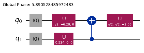
これで、回転 Gate を使った情報エンコーディングの方法を確認できました。
3.2 角度エンコーディングとパラメータ化Circuit
量子コンピュータへ情報をエンコードする特に興味深い方法の1つは、ある回転角 またはパラメータを含む量子 Circuit を設計し、関数族 を表現できるようにチューニングすることです。例として、次のようなパラメータ化量子 Circuit を考えてみましょう。
from qiskit import QuantumCircuit
from qiskit.circuit import Parameter

# Define a symbolic parameter
theta = Parameter("θ")

qc = QuantumCircuit(2)
# We applied a parametrized RX gate
qc.rx(theta, 0)
qc.cx(0, 1)
qc.draw("mpl")

数学的には、この Circuit で表現できる関数族を次のように分析することができます。
この量子 Circuit で表現できる状態の数は限られており、例えば や といった状態は表現できないことが明らかです。しかし、適切な位置にさらに多くの回転を導入することで、表現できる状態の族が広がります。
from qiskit import QuantumCircuit
from qiskit.circuit import Parameter

# Define a symbolic parameter
theta1 = Parameter("θ1")
theta2 = Parameter("θ2")

qc = QuantumCircuit(2)
qc.rx(theta1, 0)
qc.rx(theta2, 1)
qc.cx(0, 1)
qc.draw("mpl")

この場合、表現される量子状態は次のようになります。
\begin{align*} \text{CNOT}_{01} \, R_x^{\{1}}(\theta_2) R_x^{\{0}}(\theta_1) \ket{00} &= \text{CNOT}_{01} \, R_x^{\{1}}(\theta_2)\left( \cos(\theta_1/2)\ket{00} - i\sin(\theta_1/2)\ket{10} \right) \\ &= \text{CNOT}_{01}\left( \cos(\theta_1/2)\cos(\theta_2/2)\ket{00} - i\cos(\theta_1/2)\sin(\theta_2/2)\ket{01} \right. \\ &\quad \left. - i\sin(\theta_1/2)\cos(\theta_2/2)\ket{10} + \sin(\theta_1/2)\sin(\theta_2/2)\ket{11} \right) \\ &= \cos(\theta_1/2)\cos(\theta_2/2)\ket{00} - i\cos(\theta_1/2)\sin(\theta_2/2)\ket{01} \\ &\quad + \sin(\theta_1/2)\sin(\theta_2/2)\ket{10} - i\sin(\theta_1/2)\cos(\theta_2/2)\ket{11} \end{align*}この Circuit は、前の Circuit と比較してより広い量子状態の族を生成できることがわかります。特に、上記の Circuit では不可能だった や に対してゼロでない振幅を持つ状態を生成できるようになっています。ただし、この Circuit はまだ普遍的な量子状態生成器ではありませんが、特定の関数を表現するために一定の柔軟性を持つ Circuit を設計するのに十分な表現力を持っている場合があります。一般的に、独立したパラメータ(角度)を多く導入するほど、Circuit が任意の量子状態を近似するための表現力が高まります。
Ansatz と Circuit ライブラリ
このようなパラメータ化量子 Circuit は、Ansatz(問題の解を近似しようとする試行量子状態)の構築に使用できます。これらの Ansatz は、変分量子アルゴリズムの中心的な構成要素です。変分量子アルゴリズムは、量子コンピュータを用いてコスト関数を評価し、古典的なオプティマイザを使ってそれを最小化するハイブリッド量子古典アルゴリズムの一種です。これらのトピックについては後のユニットで詳しく説明しますが、今は Qiskit の Circuit ライブラリ を使って簡単な Ansatz を構築する方法を紹介します。
from qiskit.circuit.library import efficient_su2

SU2_ansatz = efficient_su2(4, su2_gates=["rx", "y"], entanglement="linear", reps=1)
SU2_ansatz.decompose().draw(output="mpl")
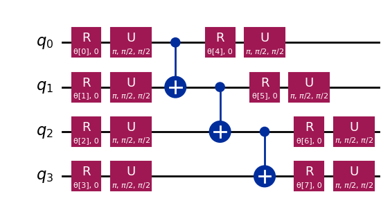
qiskit.circuit.library の efficient_su2 関数を使って、パラメータ を調整することで幅広い量子状態を生成できる簡単な Ansatz を構築する方法を確認しました。
まとめ
このノートブックでは、量子 Gate の構築からオブザーバブルの定義と測定まで、量子 Circuit の構築方法を学び、シミュレータと実際の量子ハードウェアの両方でこれらの Circuit を効率的に実行する方法を学びました。また、実際の量子デバイスを使用する際にエラーを最小化するための慎重な Circuit 設計の重要性と、特に GHZ 状態の例を通じて、より多くの qubit 数へ Circuit をスケールアップするための戦略も確認しました。さらに、振幅エンコーディングや角度エンコーディングを含む、古典的な情報を量子状態にエンコードするさまざまな手法を探りました。これらをすべて踏まえて、次のセッションに進み、量子アルゴリズムの学習を始める準備が整いました。
VSCode に Qiskit Code Assistant をインストールする
リンクをクリックして、指示に従ってください。
ボーナス:量子テレポーテーション
量子テレポーテーションという言葉を聞くと、ある場所で物体を分解し、遠く離れた別の場所に再び現れるという近未来的なSF技術を想像するかもしれません。しかし、量子テレポーテーションはそのようなものではありません。実際にテレポートされるのは物質ではなく、情報です。
量子テレポーテーションは、ある場所の qubit の量子状態を別の場所へ転送することを可能にします。この転送は瞬間的に見えますが、物理法則に違反していません。なぜそれが可能なのでしょうか?詳しく見ていきましょう!
量子テレポーテーションは、送信者(アリス)が qubit q の状態 を受信者(ボブ)に伝送するプロトコルです。これには2つの主要なリソースが必要です。共有されたエンタングルした qubit ペア a と b、および2ビットの古典的な通信 c0 と c1 です。
このプロトコルが必要とするものは次のとおりです。
q: アリスの qubit。初期状態 にあり、テレポートしたい状態です。a: 共有エンタングルペアのアリス側の半分。b: 共有エンタングルペアのボブ側の半分。c0,c1: アリスの測定結果を格納するための古典ビット。
そして、どのように動作するのでしょうか?ワークフローは次のとおりです。
q上にアリスの状態 を準備します。 検証のために のような特定の状態を作成します。- エンタングルメントを作成します:
aとbの間にベル対を生成します。 - アリスの操作: アリスは2つの qubit(
qとa)に対して「ベル測定」を実行し、古典的な結果をc0とc1に格納します。 - 古典的な通信: アリスは2つの古典ビット(
c0,c1)をボブに送信します。 - ボブの補正: ボブは受け取った
c0とc1の値に基づいて、自分の qubit(b)に特定の量子 Gate(X および/または Z)を適用します。
すべてが正しく行われた場合、ボブの qubit b はアリスの q の元の状態 になります!
量子テレポーテーションのより詳細な説明と探索、およびこのプロトコルが機能する理由の数学的説明については、IBM Quantum ラーニングリソースを参照してください:量子テレポーテーション。これは 量子情報の基礎 コースの一部です。
import matplotlib.pyplot as plt
from qiskit import QuantumCircuit, QuantumRegister, ClassicalRegister
from qiskit_aer import AerSimulator
from qiskit.visualization import plot_histogram, plot_bloch_multivector
# Define individual quantum registers for each qubit
q = QuantumRegister(1, name='q') # message qubit
a = QuantumRegister(1, name='a') # Alice's entangled qubit
b = QuantumRegister(1, name='b') # Bob's entangled qubit
# Classical register for Alice's measurements
cr_alice = ClassicalRegister(2, name='c_alice')
# Create quantum circuit
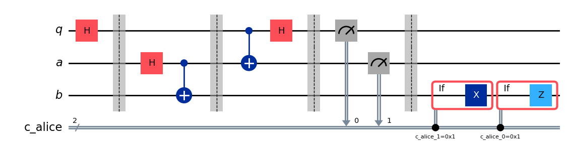
teleport_qc = QuantumCircuit(q, a, b, cr_alice, name='Teleportation')
# Step 1: Prepare message state |+⟩ on q
teleport_qc.h(q[0])
teleport_qc.barrier()
# Step 2: Create entanglement between a and b
teleport_qc.h(a[0])
teleport_qc.cx(a[0], b[0])
teleport_qc.barrier()
# Step 3: Alice's Bell measurement
teleport_qc.cx(q[0], a[0])
teleport_qc.h(q[0])
teleport_qc.barrier()
# Step 4: Alice measures q and a
teleport_qc.measure(q[0], cr_alice[0])
teleport_qc.measure(a[0], cr_alice[1])
teleport_qc.barrier()
# Step 5: Bob's conditional measurements
with teleport_qc.if_test((cr_alice[1], 1)):
teleport_qc.x(b[0])
with teleport_qc.if_test((cr_alice[0], 1)):
teleport_qc.z(b[0])
# Draw the circuit
teleport_qc.draw(output='mpl')
プロトコルを実行した後、重要な問いが生じます。テレポーテーションが成功したことをどのように確認すればよいのでしょうか?プロトコル実行後、ボブの qubit の状態を直接「見る」ことはできません。しかし、アリスの初期状態 を準備したので( を選択しました)、特別なタイプのシミュレーションを使用して、ボブの qubit b が同じ状態になったかどうかを確認することができます。
AerSimulator と save_statevector を使用して、ボブの qubit b がアリスの元の状態()になっているかどうかを確認します。このシミュレータは最終的な量子状態ベクトルを計算します。
そして、plot_bloch_multivector を使用してボブの qubit(b)をアリスの初期状態(q)と比較して視覚化します。
# Simulate the teleportation circuit
sv_simulator = AerSimulator(method='statevector')
teleport_qc_sv = teleport_qc.copy()
teleport_qc_sv.save_statevector()

# Execute the circuit on the statevector simulator
job_sv = sv_simulator.run(teleport_qc_sv)
result_sv = job_sv.result()

# Get the final statevector
final_statevector = result_sv.get_statevector()
print("Visualizing final qubit states:")
display(plot_bloch_multivector(final_statevector))
print("Note that Alice's qubits have collapsed to |00⟩, |01⟩, |10⟩, or |11⟩, while Bob's qubit is in the original state |+⟩.")
Visualizing final qubit states:
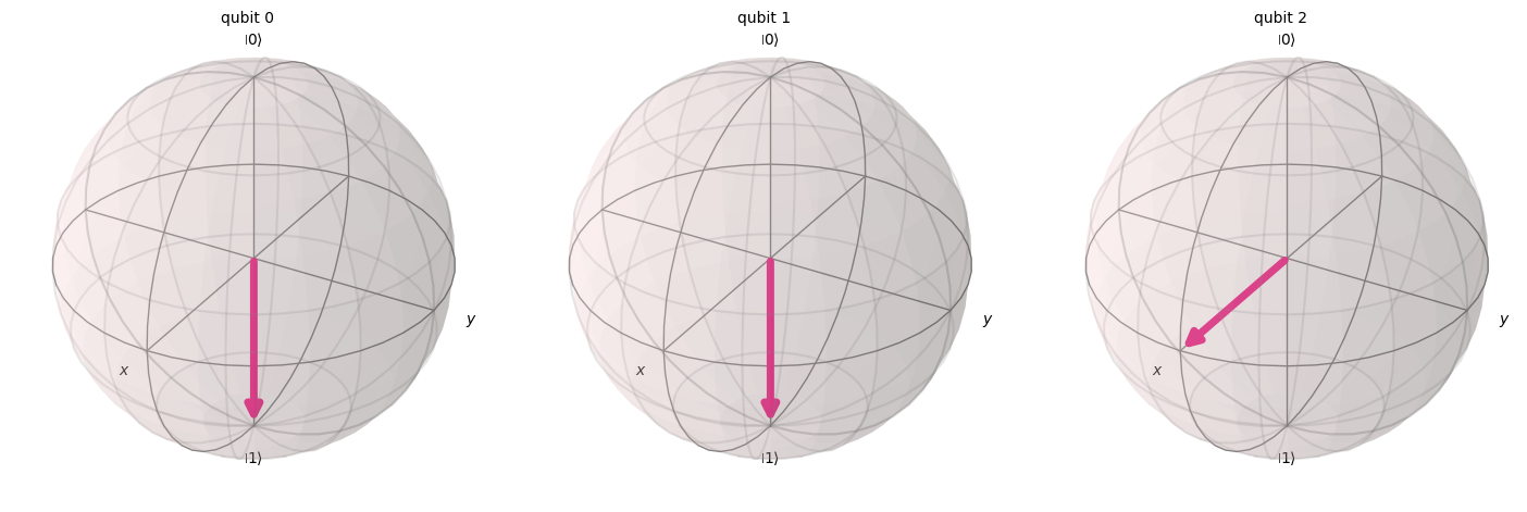
Note that Alice's qubits have collapsed to |00⟩, |01⟩, |10⟩, or |11⟩, while Bob's qubit is in the original state |+⟩.
視覚化から確認できるように、最初の2つの qubit(アリスのもの)は0または1に収縮しています。一方、3番目のブロッホ球で表現されたボブの3番目の qubit は、x軸方向を向いており、 状態にあることを示しています。これで、量子テレポーテーションプロトコルの実装に成功しました!
まとめ
ここで、私たちが達成したことを簡単にまとめておくことは有益です。
- アリスは未知の量子状態をボブに伝送しました。
- 物理的な粒子は転送されていません。
- アリスの qubit 上の元の状態は破壊されており、これは複製不可能定理に従っています。
ただし、量子テレポーテーションには依然として古典通信(アリスの測定結果をボブに送信すること)が必要であり、そのためこのプロセスは光速を超えた情報転送を可能にするものではなく、既知の物理法則のすべてと完全に一致しています。